Scripting For All Summer '21

Minterm Expansion Principle

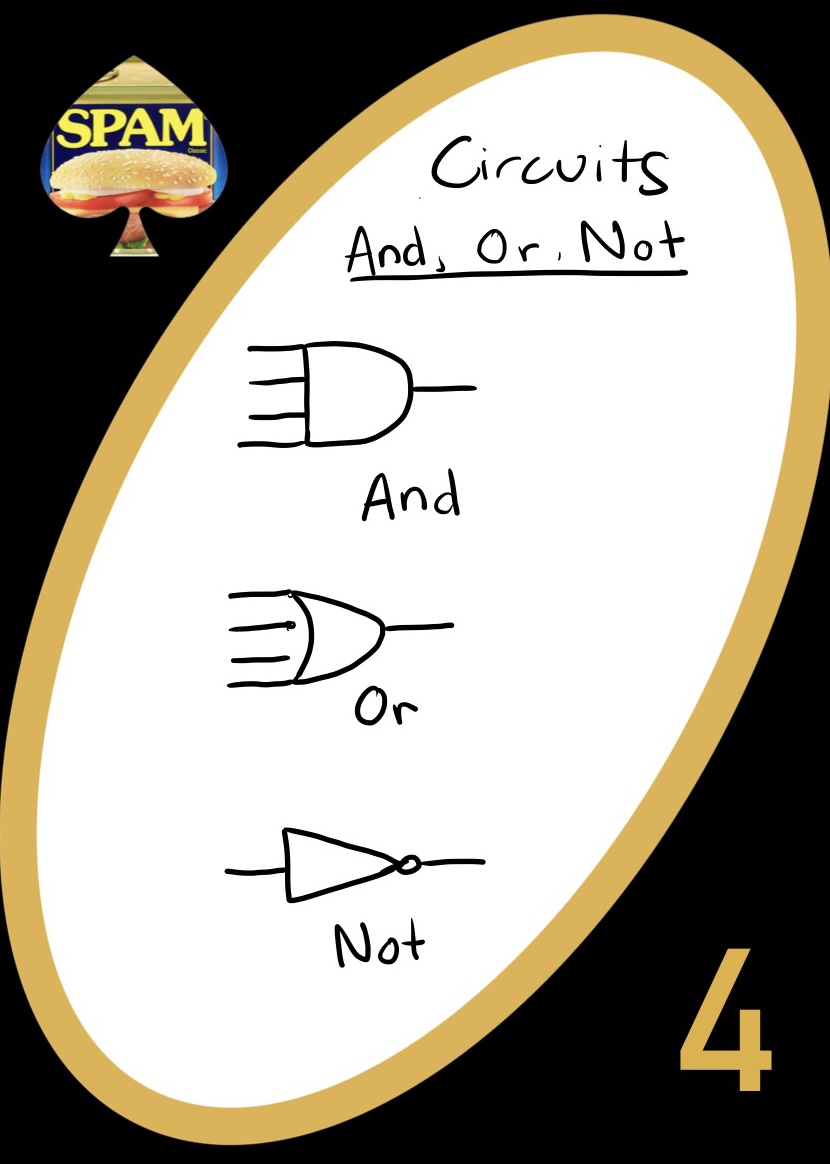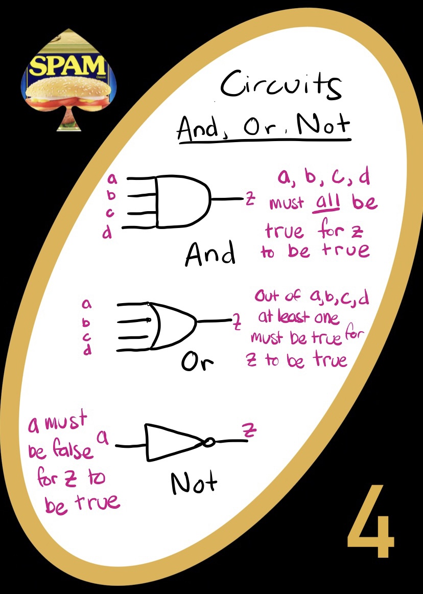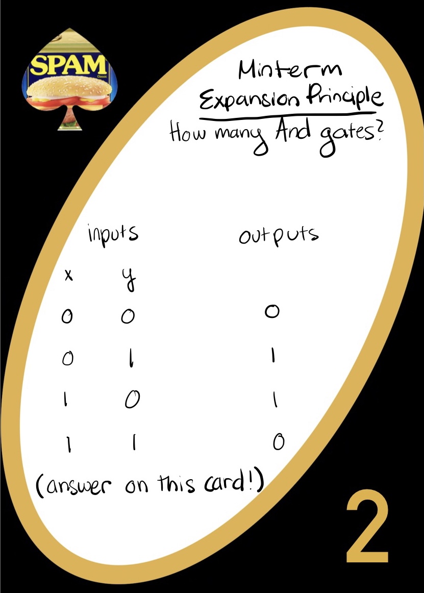
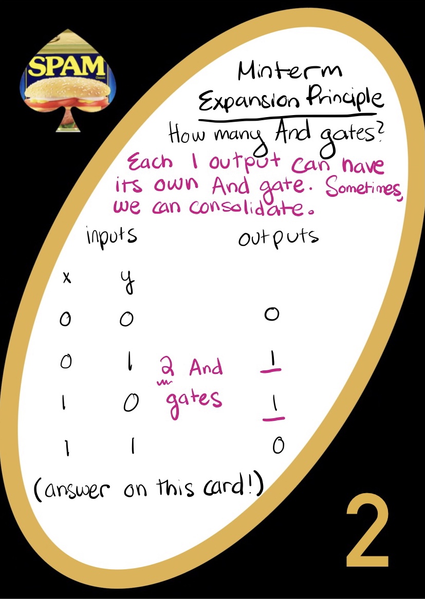
Given a boolean function — represented as a truth table — how can we construct a machine that computes that function? The answer is combinational logic — a technique for using gates to implement boolean functions. A minterm is an AND gate that is connected to all its inputs directly or through a NOT gate. Minterm expansion (sometimes called the “minterm expansion principle”) is an algorithm for transforming a truth table into a circuit:

Look at all possible combinations of values for the inputs to the function: For each combination of values that should cause the function to output 1, build a minterm that outputs 1 only for those input values (and 0 for all other input values)
OR all the minterms together

The resulting circuit implements the truth table.

Click here for more info

Image Compression

Take a closer look at the bottom of the pop tarts box. Can you read the text? I certainly can’t! This is because the image has been compressed: a few times, actually. As part of CS5, everyone gets to code an image compression algorithm. To do this, we need to think about any image we’re given as a string of binary digits, like this one: ‘01000010110101001010101’

To compress an image, we literally compress the binary string representation of the image. For our algorithm, we have a few steps to think through.

We need to think about our string as a way to carry simple information. In this way, we are going to re-write that information. Strings with lots of repetition should be easy to condense. We can write those repeated strings as a product of two things. (Hint: consider multiplying the character we are repeating by … something … )
Once you’ve figured out how to write a repeated number as a product, we can make it regular. We can decide how many times is the most that we can repeat a number - writing this in binary, of course. All the other numbers we’ll need to “pad” with front zeros
Write the code! We are going to iterate through an entire binary string recursively, and decide how to express certain repeated values as one string that is (hopefully) shorter. Consider writing helper functions that: count the number of repeated 1’s/0’s, convert base 10 integer counts to binary counts.

Circuits

Use the circuits site!

There are several important gates that are used in logic circuits

AND gates output True if all inputs are True. Otherwise they output False
OR gates output True if at least one of the inputs are True. Otherwise they output False
NOT gates simply reverse the input! Inputting True outputs False, and inputting False outputs True

Binary to Base-10

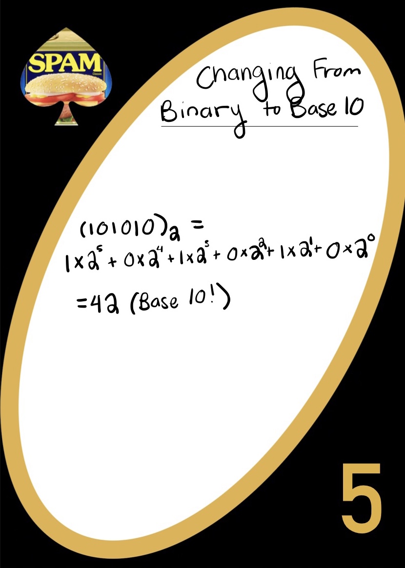
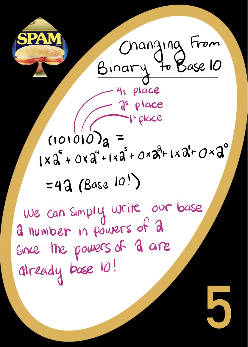
In python, there are built-in functions to convert between binary and base-10. For example, bin(42) will return the string "0b101010" (the "0b" is python's way of marking a binary number). The int() function can convert from an arbitrary base to base-10 by passing in a second argument. For example, int("101010", 2) parses the string as a binary number and returns 42

The Stack

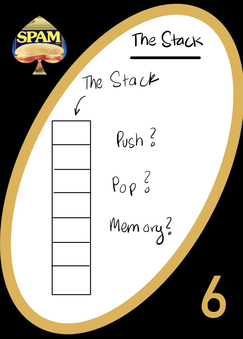
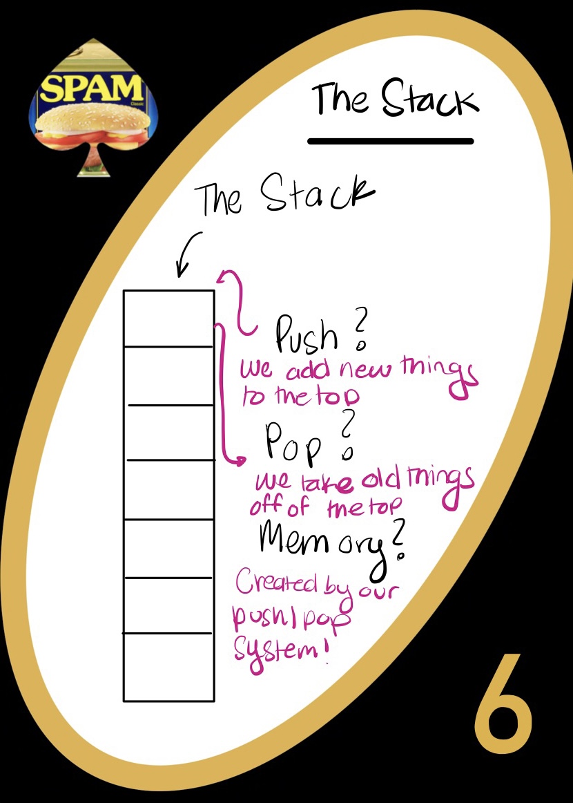
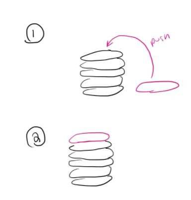
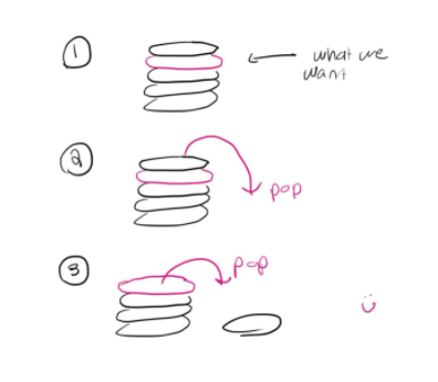
The stack is where all of our stuff gets stored! This is where we get computer memory from - stack pointers let us traverse (almost literal) stacks of information. We put “elements” or information into the stack, and it changes size when we do. There are two main methods that we need to consider when learning about the stack:

Push means we are putting a new element onto the top of the stack
Pop means we are taking an element from the stack

HMMM with Wally!

Finite State Machines

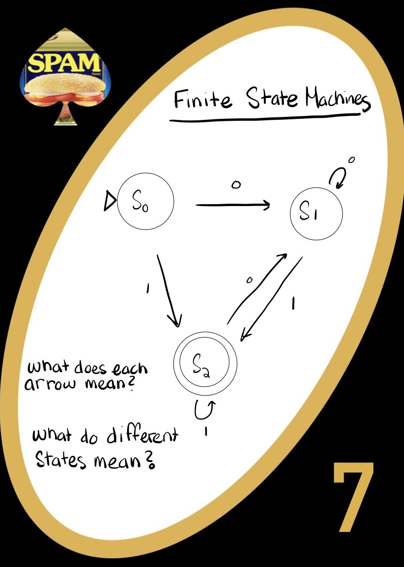
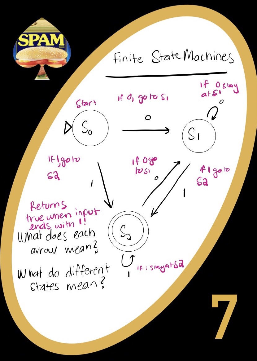
A state is a situation of the ‘system’. I can have a light switch that is on or off, then there are 2 states. We represent these states with circles in our FSMs. A state can either lead to a 0 or a 1 (for us). Either that state happens and triggers one thing, or that state happens and triggers another thing.

You can stay in the same state
You can move to a new state

Something that has 2 circles just means it returns TRUE when you get to, and stay, at that state. Your goal is to design a system that returns true every time when you want it to return true. Want more practice? Visit the CS5 site to play with more FSMs!

Branching Recursion

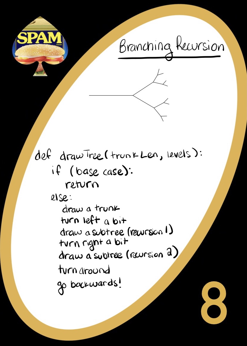
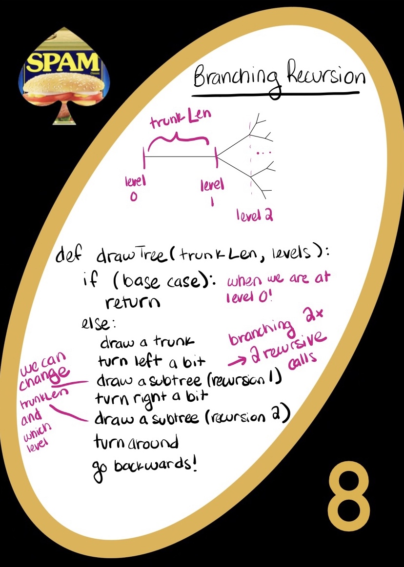
Branching recursion is just like normal recursion, except that different cases end up with different recursive calls. It can help to picture a recursion ‘tree’ - each different recursive call makes its own branch. This is different from normal recursion in that you need to check two different recursive calls to get the job done.

The example on the card draws a recursive tree - it branches twice each level, just like our recursion! On the pseudocode, you can see that the subtrees (left and right) are happening simultaneously, and each represents a different path to get to the base case. The power of the recursion here is that our computers can make this tree, see the best choice out of all the choices (when we care about outcomes), and come back to the start of the tree without breaking a sweat.

We might want to use branching recursion when there are two distinct paths to take in a problem. Besides trees, some examples include exact change, scrabble outcomes, or even the most recent common ancestor in biology. The thing that all these seemingly different problems have in common is that they ask for a specific result, and there are two different outcomes at each choice. We can look closer at exact change: if we want to make a total from a pile of coins, we are always either using or losing a coin. Useit or Loseit are then each their own outcomes: we can recurse through both for every single coin until we get a set of combinations that gets exact change for a total!

Classes vs. Objects

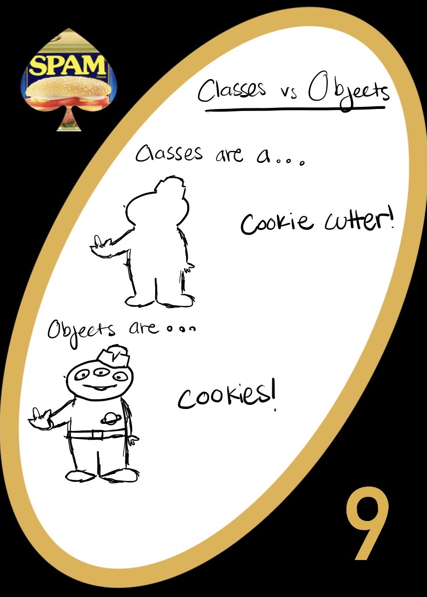
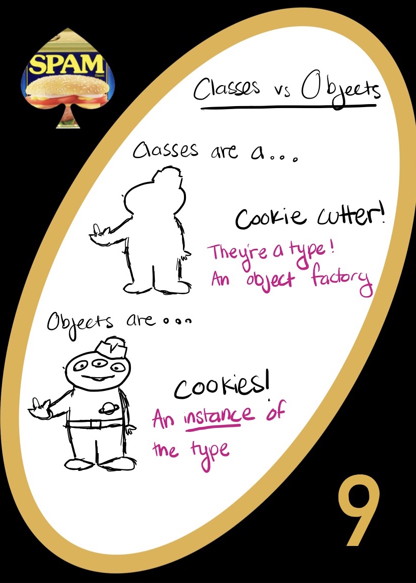
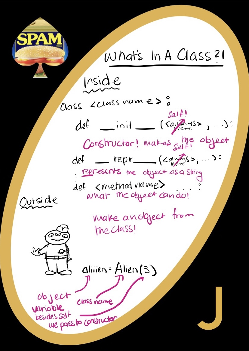
Classes and objects are similar (which is sometimes confusing). However, classes are different from objects.

Classes are ‘cookie cutter’ that lets you make many objects of the same type. Those objects should all have things in common, since they’re specified by the class!
For example, I can have an Alien class that makes three eyed aliens, klingons, and daleks. Classes are like object making factories!

Onjects are a single instance of a class.

Objects are the real things that have attributes that you specify with a class in order to make the object
If our class is Alien, the alien that you make with that class is an object! I can make a three eyed alien named burt who is an object that belongs to the Alien class. I can also make him a klingon friend named (or in English, chad) who will be an object that belongs to the Alien class. Finally, we can make Davros who is a Dalek, and is also an Alien
When we make objects from a class, we are saying that they have attributes that we specify with the class

Example: Classes and Objects

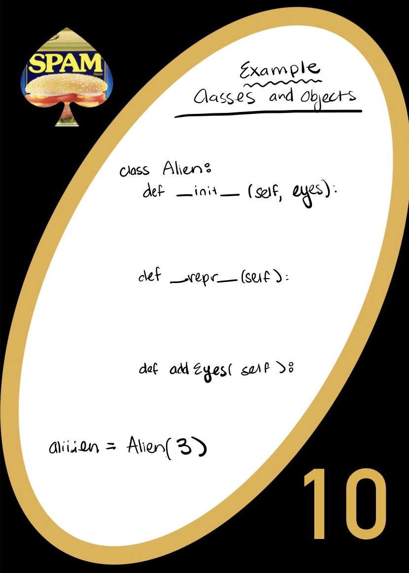
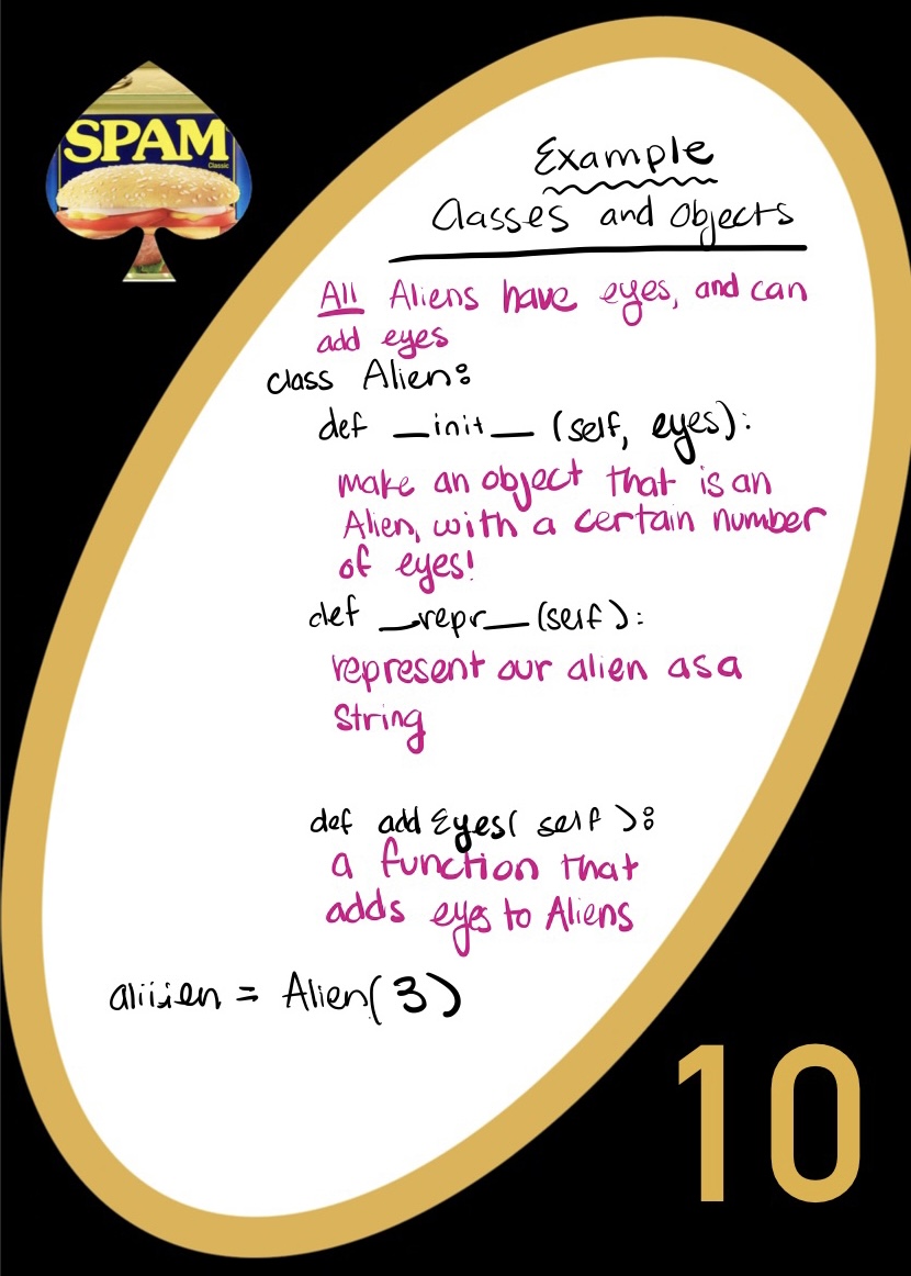
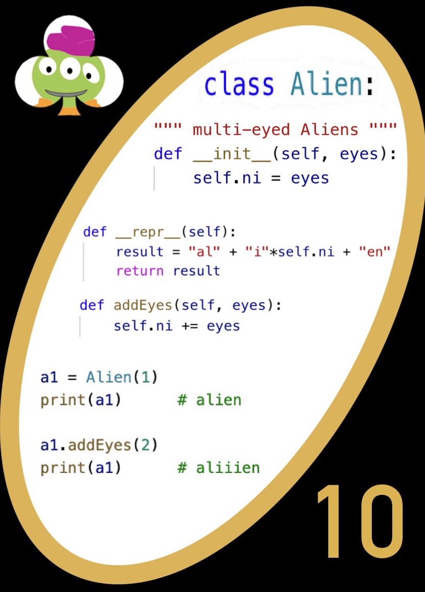
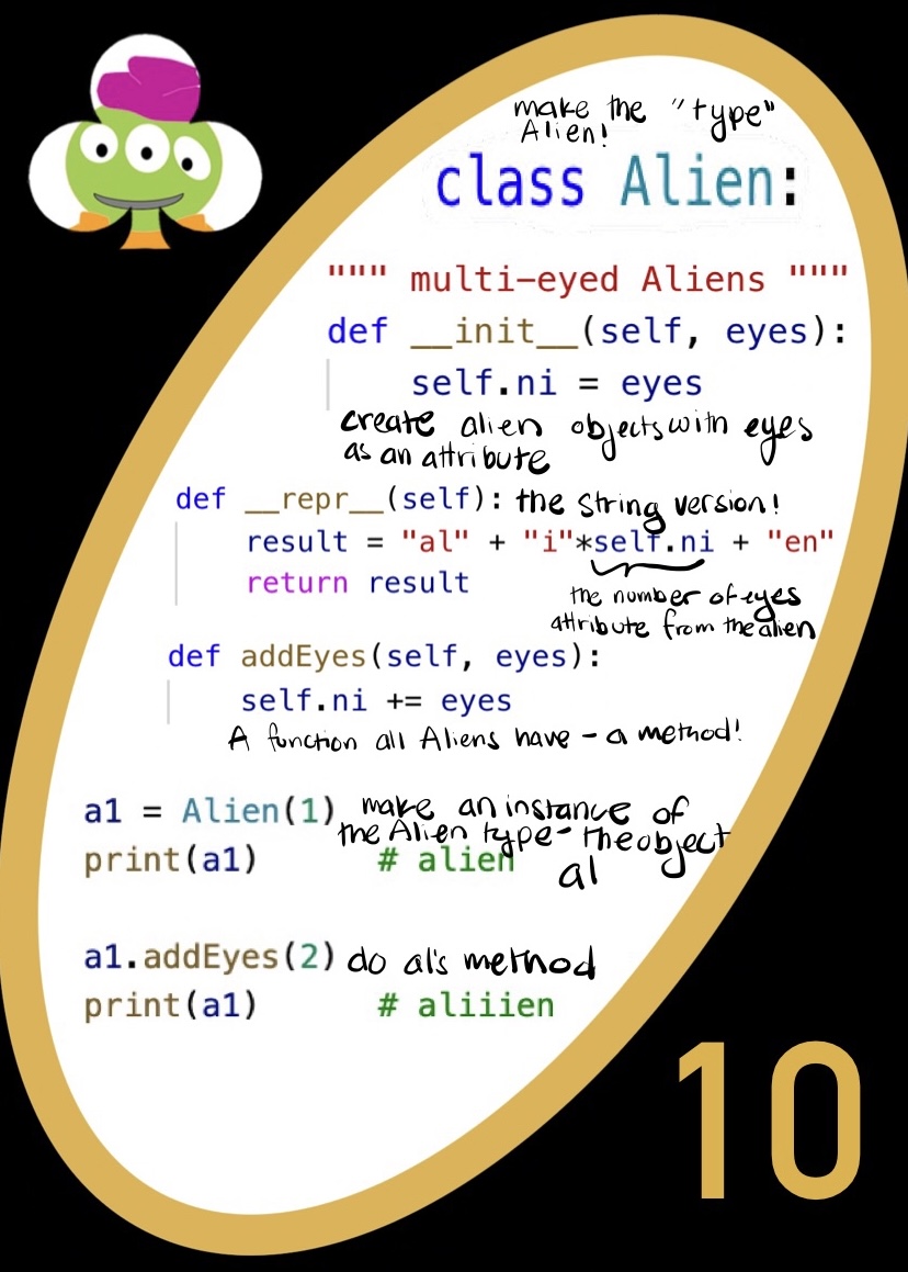
Let’s write an example Alien class that makes a 3 eyed alien object. First, we can note what we want all aliens (or objects belonging to the Alien class) to be able to do. Aliens should be able to count to 42, have names, and they can have 3 eyes. Since these are all things that every alien can do / have, we can write them in our class.

In our example, each time we make a new alien, we need to specify the Alien attributes in the constructor. To our constructor, we can send the number of eyes our Alien will have, and their name. Then, when our Alien gets “made”, it will have the attributes we specify! Next, we need to write the repr function. This function represents our Alien of choice as a string! This one is left to your imagination.

Onto methods! The next thing we need to do is say what our Aliens can do. Here, we can write a method (which is just a fancy word for function) that specifies how our Alien can count to 42! Aliens will need to do other things of course, but for now, let’s make a sample alien. We get to make a 3 eyed alien. This Alien is stored in the variable instance aliiien, and we use the class Alien, specifying aliiien’s name (“aliiien”) and how many eyes aliiien will have. All Aliens can count to 42, so we don’t need to say whether aliiien can count to 42.

That’s it! You’ve made an Alien!

What's in a Class?!

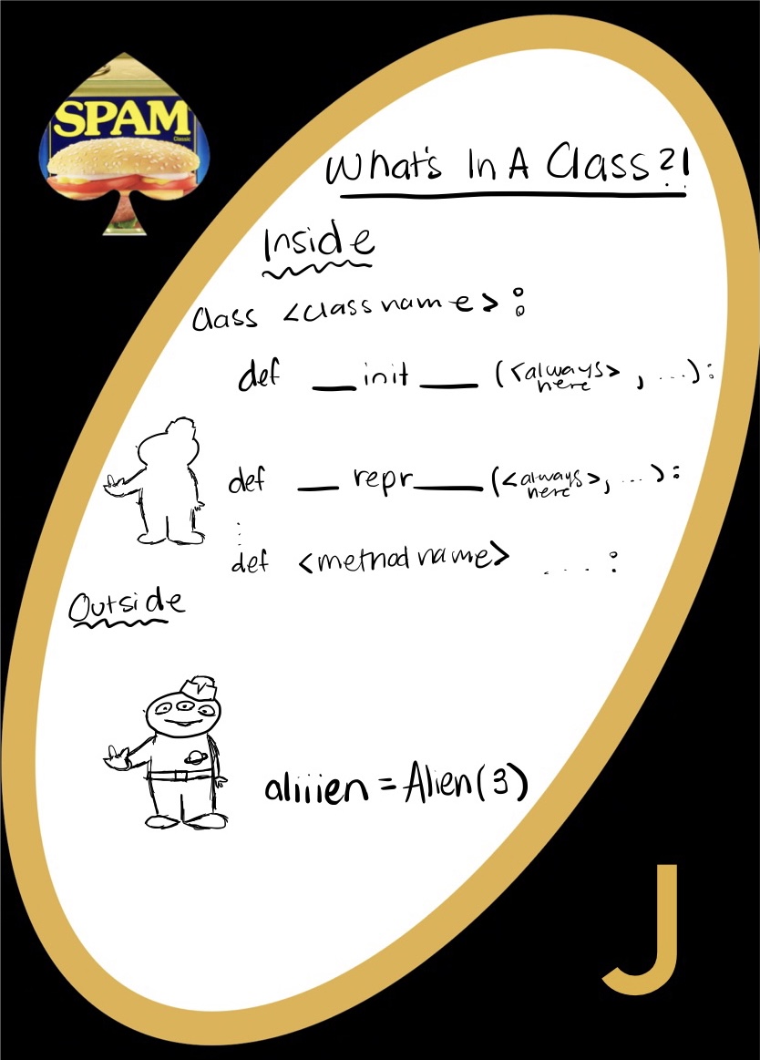
All classes have a constructor, a repr function, and maybe some methods.

Constructor

This is where you actually make the object - self! Self is different based on what object you are making. The class treats self as the same
May need to specify what attributes every object will have (ie, do all aliens have eyes, etc)
You always need to write __init__(self, *kwargs)
Inside, you specify how the variables you pass in get assigned to the object

Repr

This function returns a representation of the object that we can see (as a string)
This should return different things based on what you need your object to do
You will always write ___repr__(self)

Methods

Methods are just functions that all objects of a class can do. Maybe all aliens can eat spam. Then we would write a method eatSpam(self) that says how aliens eat spam.
When we call methods outside the class, we need to know what object is doing the method and all the variables we pass into the method (besides self, since self is the object)
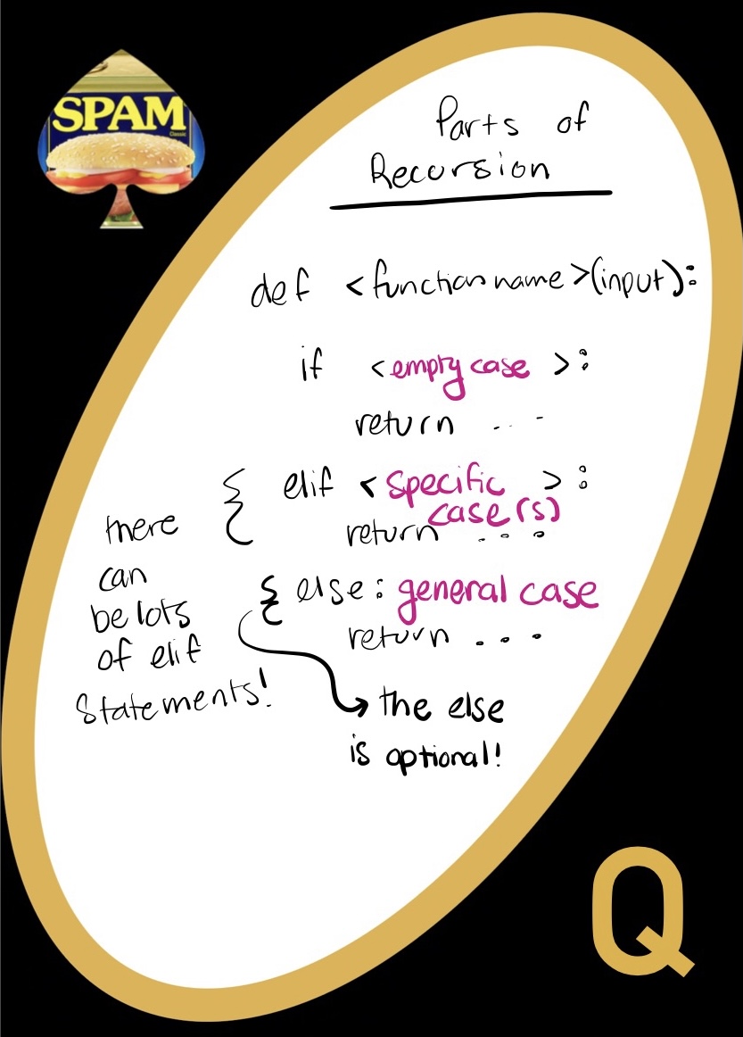
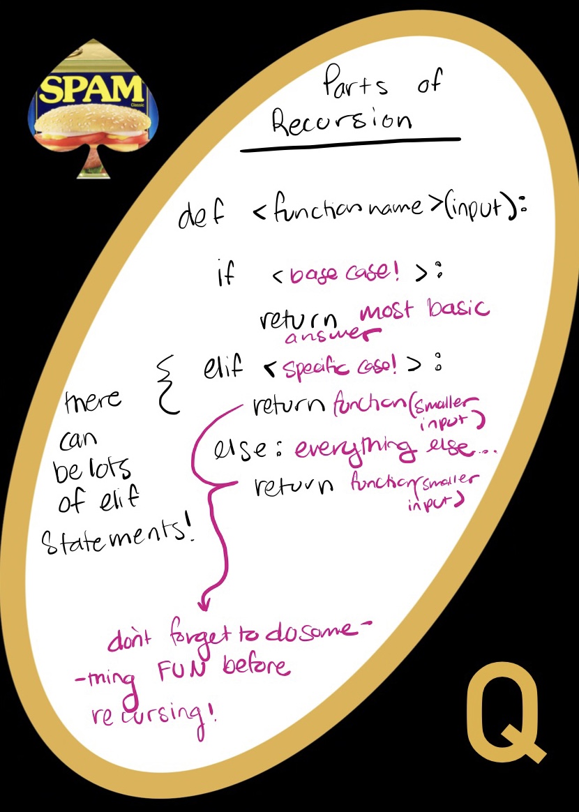
We do this by saying object.method(variables). Look familiar?

Parts of Recursion

Recursion always has at least two parts, and it usually has three!

Base Case

The base case tells us when to stop
When we get to the end of our input what should we return? Sometimes you will be inputting a string and want an integer (say, if you wanted to count the i’s in aliiiiiiiiien) so we’d check whether a string is empty and return a number, in this case, 0

Recursive Part

We can think of the recursive part as the actual stuff we want to do to our slice of our input. Sometimes this is broken into multiple steps; you always handle the specific case first, and then everything else
For example, if we wanted to count how many i’s there are in alliiiiiiiiiiiien, we would take each letter at a time. We would ask our function: is the first letter an i (specific case)? For every other letter, we just skip it and keep going down the string (the general case)
In our recursive call, we will always handle one piece of information first, and then let our own function do the rest, with all of this stuck together by some operation glue
In our count i’s, we take one letter, check if it’s an i or not, and add the result to the function running ON EVERY OTHER LETTER besides the one we have just handled
If you do this enough times, you get to the end, which is our base case!

For vs. While Loops

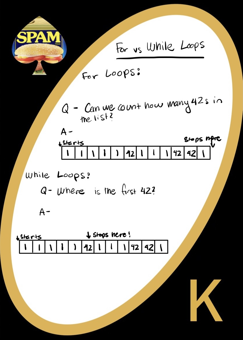
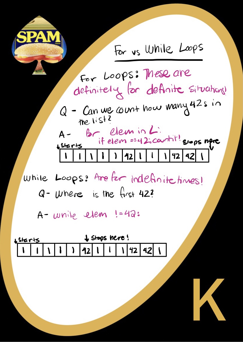
For loops and while loops are pretty similar! In fact, you can write every single while loop as a for loop.

for loop

We want to use a for loop when we know where our testing is going to end.
If we wanted to go through an entire list counting how many 42’s we have, we know exactly how long the list is. So we can say, "for every element in the list, do this thing"

while loop

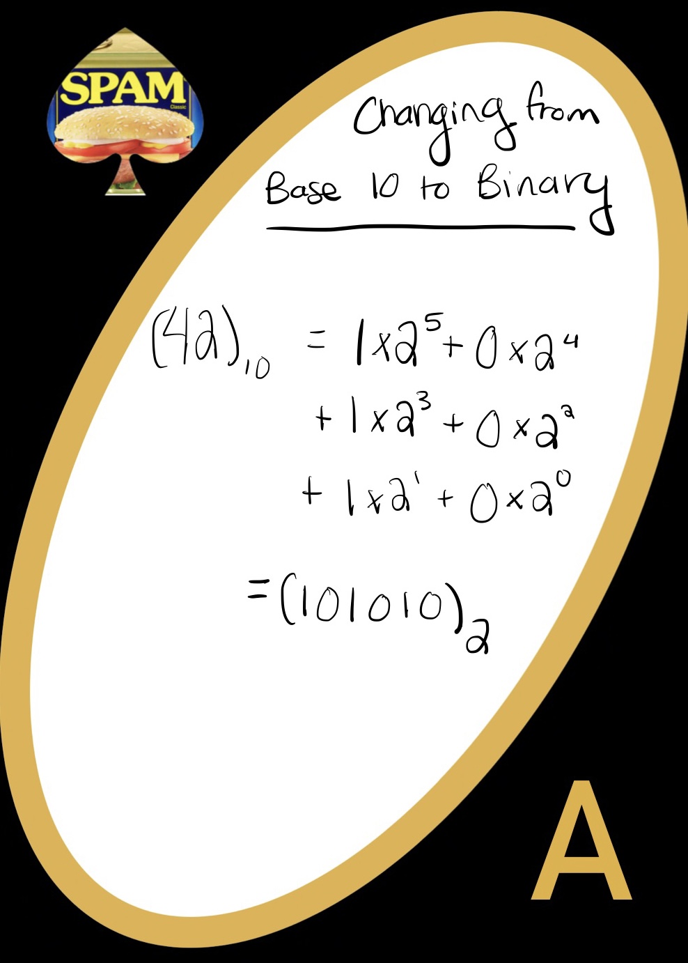
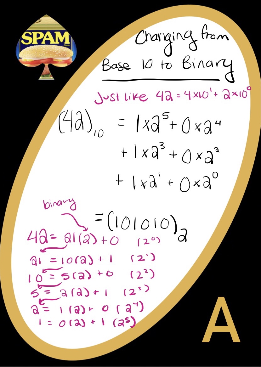
While loops are for indefinite endings - when we don’t know where in a situation we want to stop
If we took the same list as before, but asked a different question, we could use a while loop. Let’s ask: How many 1s until we hit a 42? In this case, we don’t know where the first 42 is. We can write, while our list doesn’t have a 42, keep going down the list

Changing to Binary from Base-10

To get a number into binary, the question we’re really asking is: how many times does 2 go into our number? How about different powers of 2? We can answer this by dividing by different powers of 2. If we start by dividing the number by 2, we can count how many times \(2^0\) is in that number (it will always be either 0 or 1). If we divide by 2 again, we are counting how many times \(2^1\) is in that number. Let’s write out this process:
Explanation
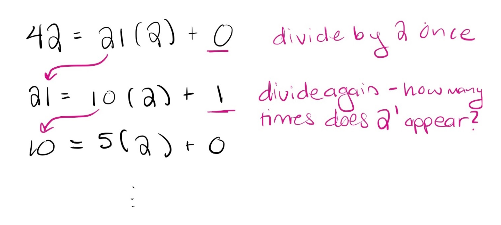
We’ve BASE-ically just written out which power of 2 we multiply by a remainder! This is our number in base 2. If you want to apply this to code, consider recursion. Every time we divide by 2, we are making our number smaller and smaller. We are keeping track of what is left in that division. If we do this until the number gets to be 0, we have reached a base case. We can then add up those digits and - voila! You have a lovely base 2 string of 0’s and 1’s.

List Comprehension

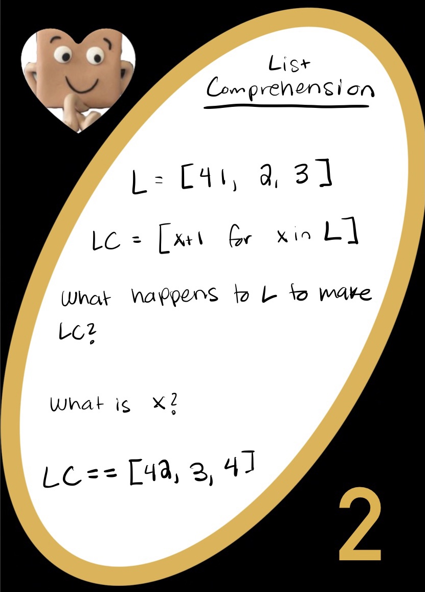
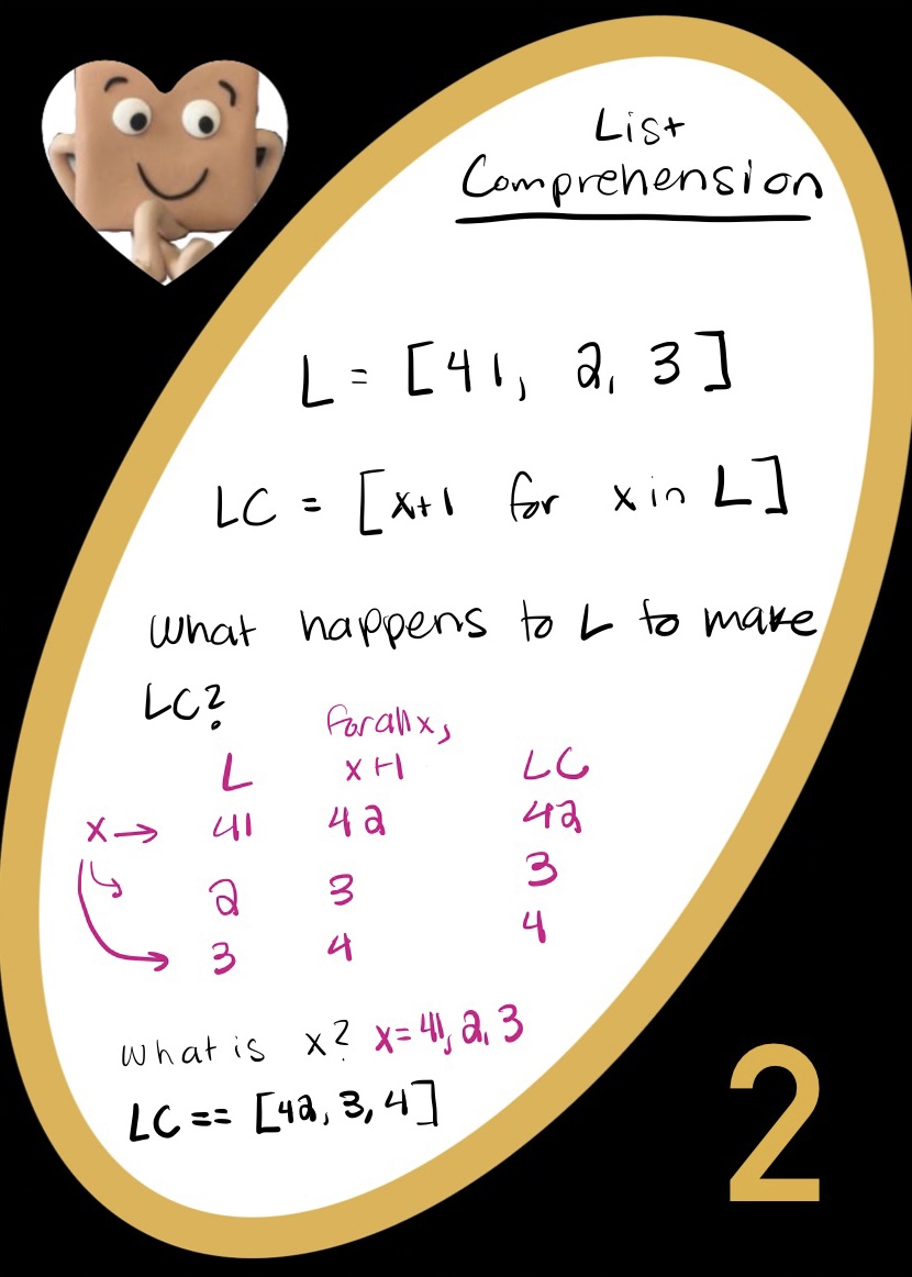
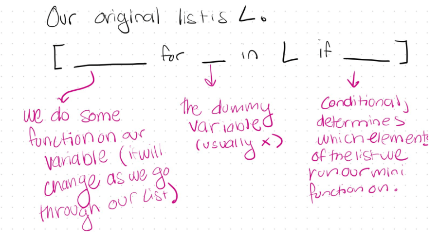
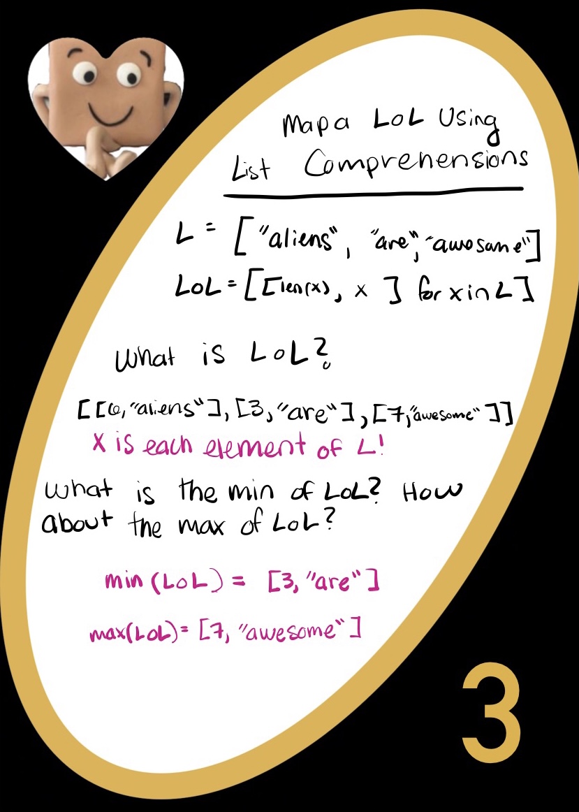
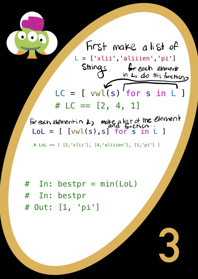
When it comes to list comprehensions, what’s really happening is that we make a mini for loop, all in shorthand. We can divide a LC into general parts: Explanation
The first part is the function or operation we are running on each element of our list to make a new list comprehension. The second part is the iterator, or what we use to go through the list. In a list of words, we would say for word in wordL, as an example. The final blank is the conditional. It filters what we add to our new LC. Maybe we only want even numbers in an LC. For this, we could use a conditional , if x % 2 == 0 to check whether x is even.

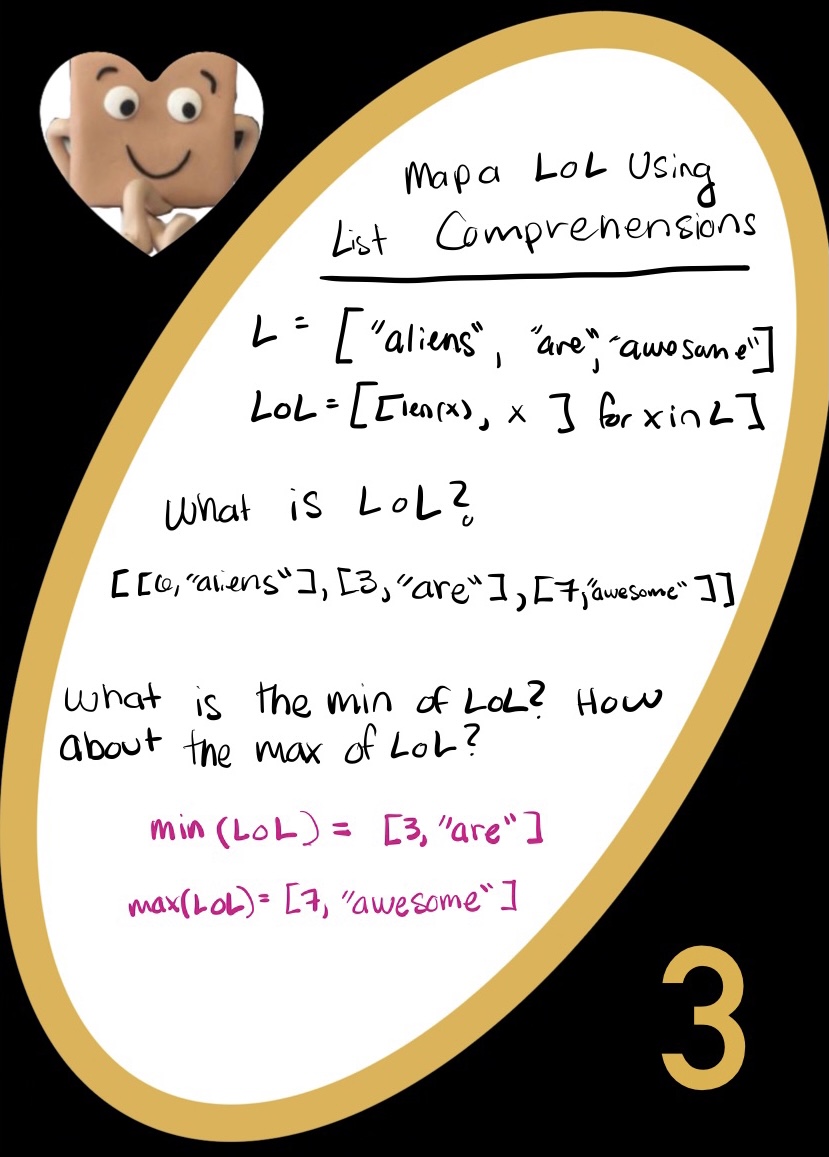
Map a LoL Using List Comprehensions

This is the same as the list comprehension, except now rather than add just one x to the list we want to return, we are adding sub-lists. We get to decide what those sub-lists are. Usually, there are some pairs, in which one value is x and the other is a function on x. This lets us pair x’s and some value we get from x, while having repeats. Remind you of anything? That’s right! Dictionaries! Dictionaries are very similar to lists of lists, except that they make use of built-in python functionality for more complex lists. LoLs let you pair ambiguous values without specified keys, if that’s how you want to think about it. They can also be easier to work with than dictionaries. Imagine taking the max of values in a dictionary: kind of hard, huh? To take the max of a LoL, we just have to make sure that the numerical value we care about is in the first spot in every list: then we can simply say max(LoL), and we’re done!

Keeping Track of Slicing

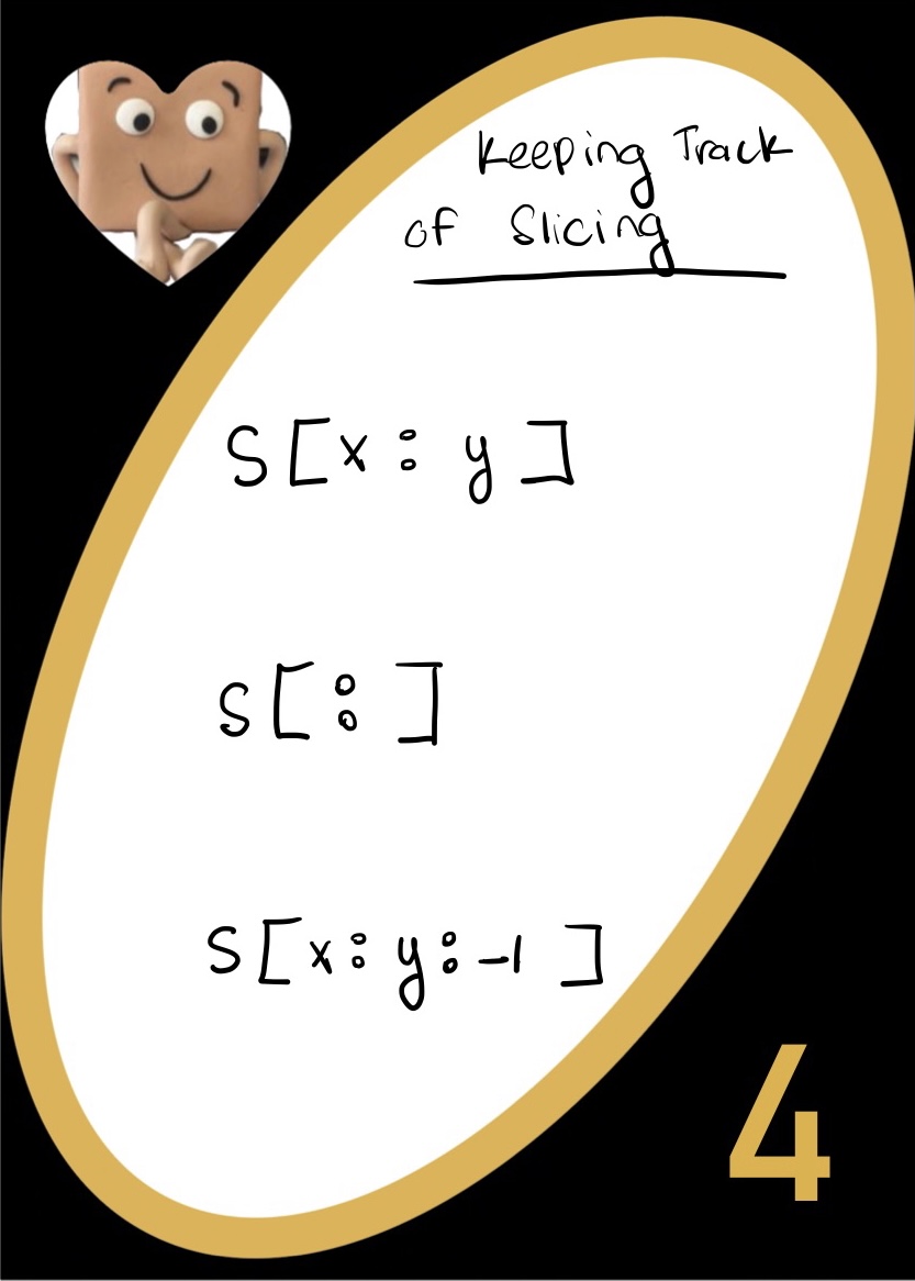
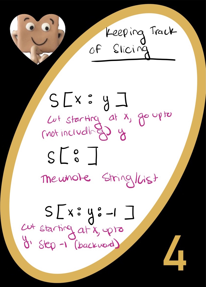
You can use brackets to slice strings and lists. For example, let S = "Harvey Mudd College"

S[7:11] is the string "Mudd"
S[:] is the string "Harvey Mudd College"
S[9:6:-1] is the string "duM"

Python also allows you to use negative indices where the last element is index -1

S[-12:-8] is the string "Mudd"
S[-10:-13:-1] is the string "duM"

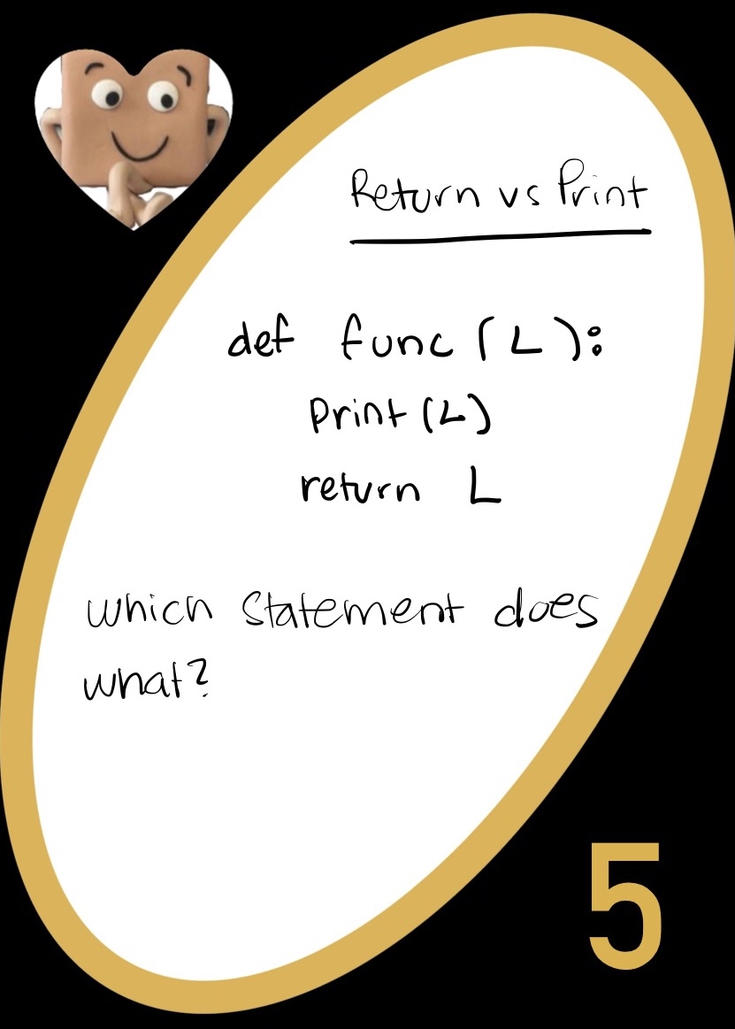
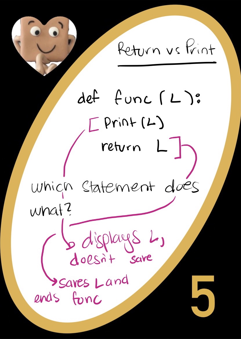
It may be difficult to get the hang of slicing rules, but with some practice you may come to appreciate some of the strange quirks. Try out our slicing website

Return vs. Print

Both return and print can (but don’t always) display whatever you’re passing in to your terminal. There are important differences, though.

Print

Print is a function that is built into python - when you call it, you pass in the thing you want to print. So, we write print("Hello World")
Print doesn’t last: It simply displays what is already there and does not store anything.

Return

Return doesn’t display anything, unless you are returning a python function that will automatically display.
Return is how we end functions: it is effectively assigning your function’s output to something, once you call the function.
This is where we see the big difference - return does store something (the output of your function) while print can simply display something.

In CS5 we are lucky enough to play Conway's Game of Life! (see slide 47 here) There are a lot of cool patterns you can create in the game, and it turns out that not all patterns are stable. (check some patterns out here) The slipping stripe reaction is a famous example of patterns that seem to be stable, but aren’t. Want to figure out why? Well, you may need the rules of the game of life, some for loops that index 2D arrays, and a way to create new generations of cells based on the old generation.

Running Recursion

Suppose we are recursing on a list L. When we are taking 1 step through the list at a time, we can expand our recursion.

We start with: function(L)
Each time we recurse, we are going to be handling L as it’s first entry and then the rest of L. We can write function(L[0] + function(L[1:]))
We can keep doing this ... function(L[0] + function(L[1] + function(L[2] + function(L[3:] ... )))
Eventually we will get to some base case, that is the end of L. That means we can unravel our recursion: the base case gets plugged into the nested functions! function(L[0] + function(L[1] + function(L[2] + function(L[3:] … + function([ ])))) or function(L[0] + function(L[1] + function(L[2] + function(L[3:] … + base case)))

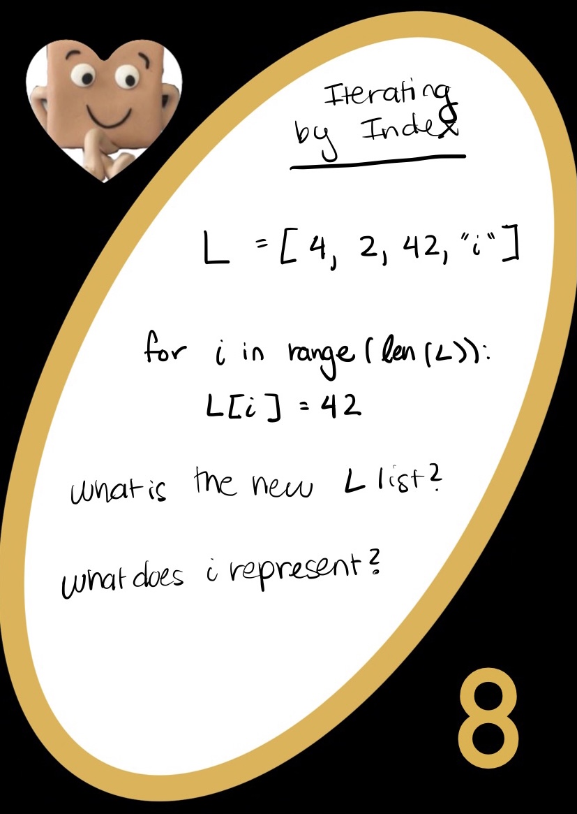
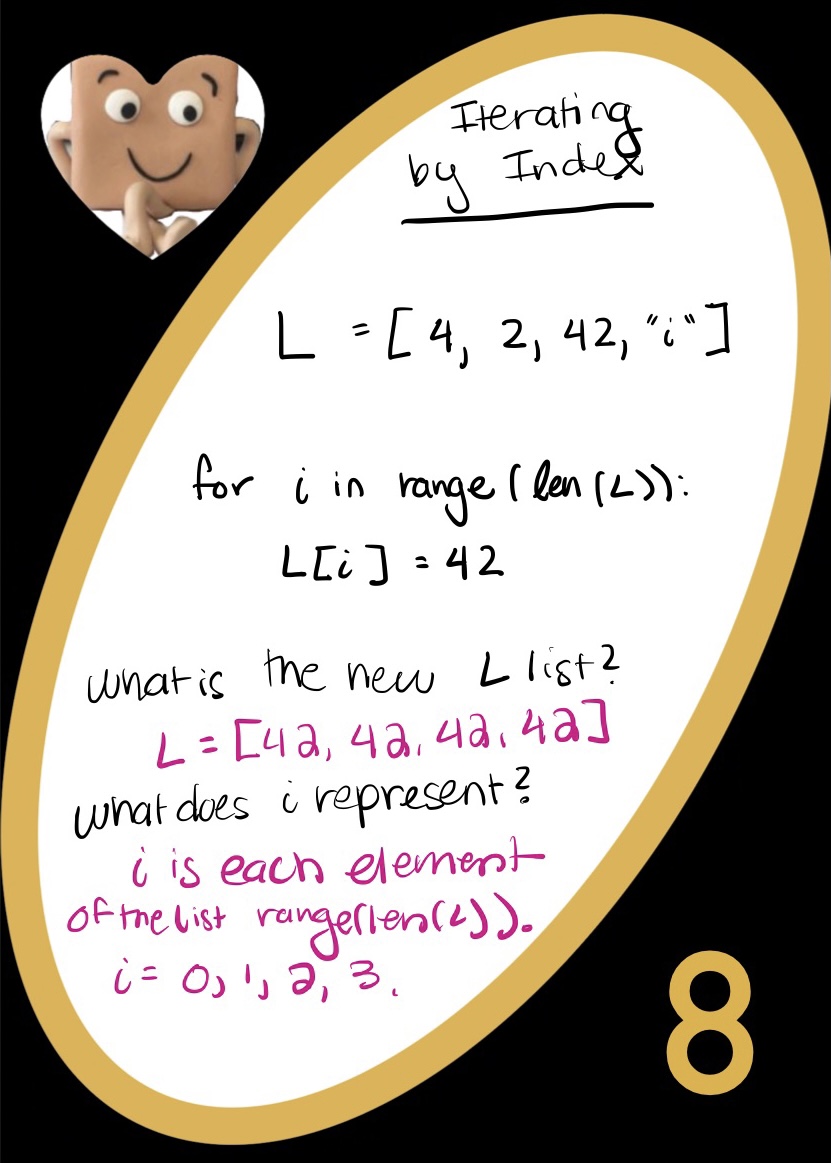
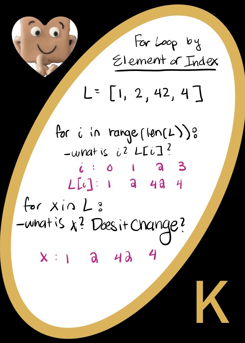
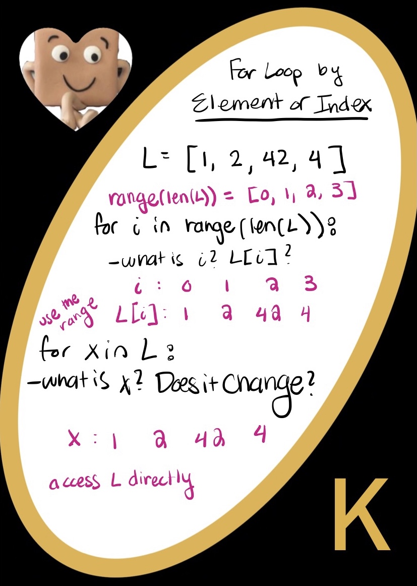
Then we step back through our calls until we end at the start of the list. Recursion, check!

Iterating by Index

The first type of for loop that we will often come across is a loop iterating through something by index. We usually write this as for i in range(...):

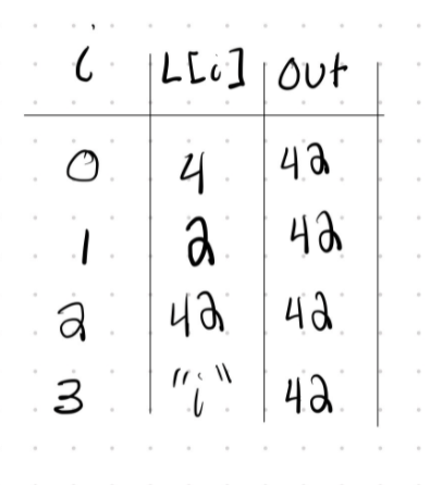
We have 3 values to keep track of : i, L[i], and what we are going to do to i or L[i] inside the loop. Since we are iterating over a range, we are basically checking every value of i between 0 and where the range ends (non inclusive). Explanation

We can write out our i values
L[i] is the value in the list at the corresponding index
Lastly, we set each L[i] to be 42, which is our output!

Indexing 2D Arrays

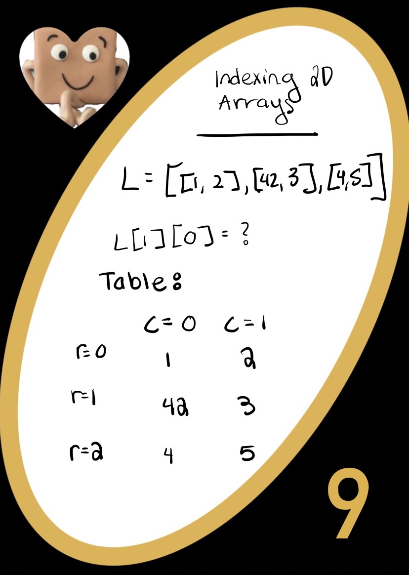
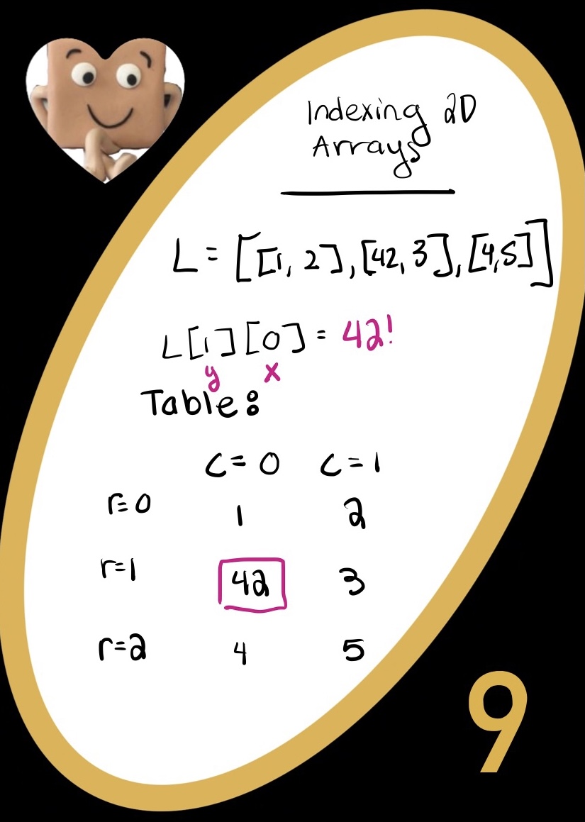
When we index 2D arrays, we can think of them as lists of lists. Naturally, to get to one of the inner lists, we have to specify where that inner list is in the outer list.

We can also turn these lists into a grid by stacking them. Now, we can see that to get to the ‘x’ value, we have to index the ‘y’ value first! From this, we can say L[y][x] to get to the (x,y) point on our grid, or for the ith element and the jth element of some list, we can index L[i][j]

Slice or Index: String?

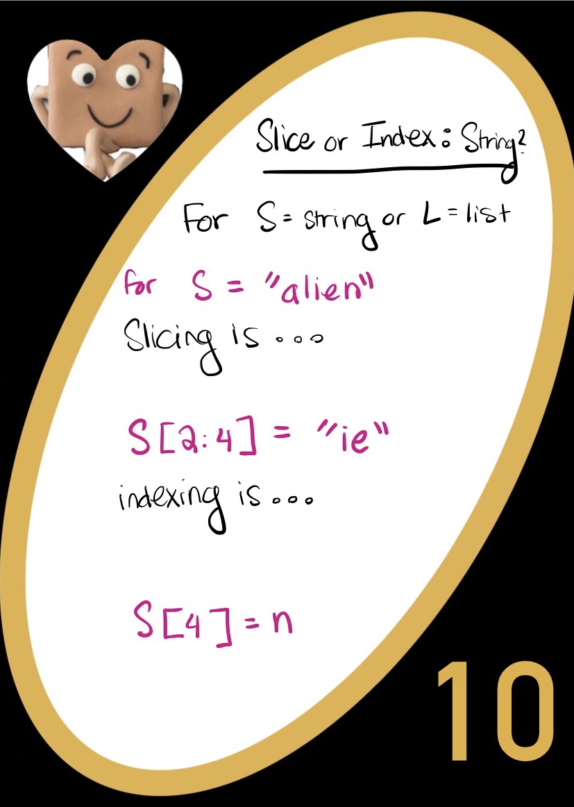
Slicing is when we are taking a chunk (or slice) of some string/list. That slice will therefore also be a string/list. This can get tricky, since S[0:1] is still a slice of a string, even though it is a slice of only 1 element.

Try the slicing website

Indexing is when we are fetching what is INSIDE the string/list at some depth into the string/list. When we say S[0], we are saying go to the 0th spot in the string S and fetch the value at that spot. This means that we are going to get whatever is inside that point! It will not always be a string or list: in fact, most of the time it is not a string or list.

If, Elif, Else... What's Different?

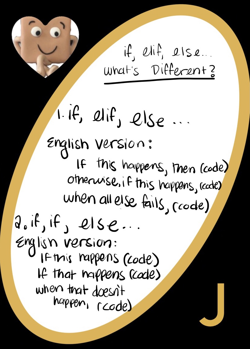
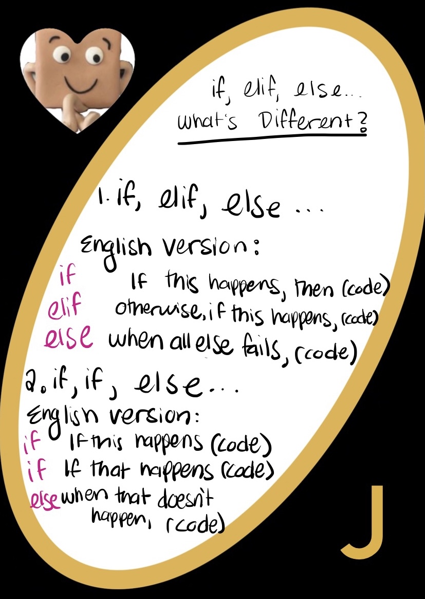
Let’s rephrase these coding words into English

if

If this specific case happens, our code will do (what you want it to do)
If statements can therefore happen independently! They are checking specific cases, not linked cases!

elif

Otherwise, if this specific case happens, our code will do (what you want)
Elif statements come after an if statement, and they are linked to each other and the if statement they belong to. This is because they are checking specific cases that happen when another specific case has not happened.

else

When all else fails, our code will do (what you want)
Else statements must also be paired with an if or elif if group. This is because you handle a specific case, and then every other case. You must handle the specific case first.

Finding Things in a Dictionary

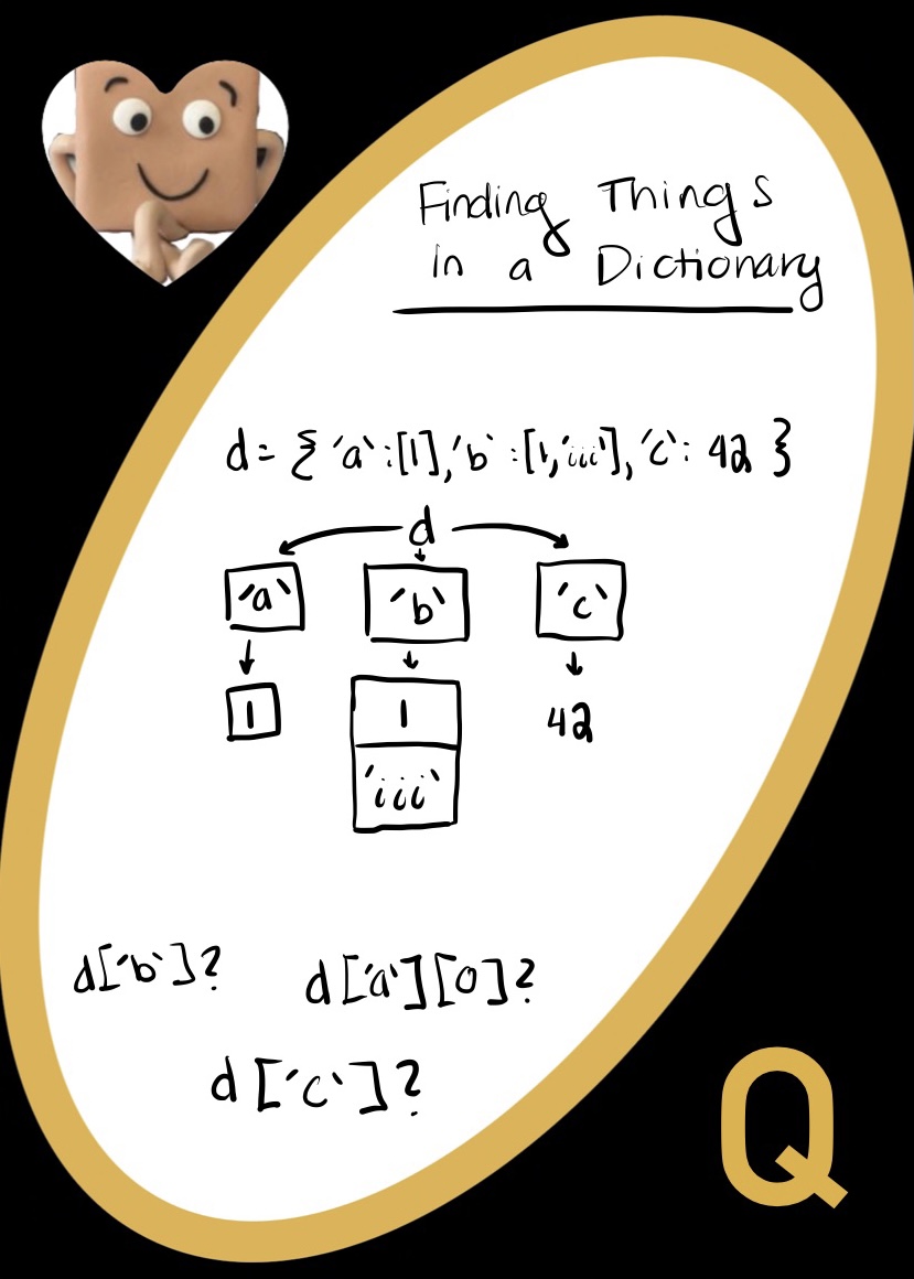
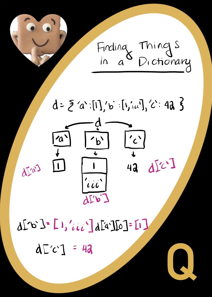
There are lots of ways to go through a dictionary. For example, let d = {'a': [1], 'b': [1,42], 'c': []}

The most common way is to search by key. Similar to indexing a list or string, you can use brackets to access the value of a key. For example, d['a'] is [1]
You can use the keys() method to view the keys in a dictionary. d.keys() returns dict_keys['a', 'b', 'c']. You can also list-ify this object to easily access the keys
You can use the values() method to view the values in a dictionary. d.values() returns dict_values[[1], [1,4], []]. You can also list-ify this object to easily access the values

For Loop by Element or Index

The first situation is looping by index. We have created a whole separate list (range(len(L))) that consists of the numbers [0,1,2,3]. We are then going to set some i (for index) equal to 0,1,2 and 3 in turn until we are done. Each time, we will do what is in the loop. We are going through our for loop by index.

The second situation is looping by element. Rather than make a new list, we instead go through each thing in L. Since L has numbers in it, elem is going to be 1,2,42, and 4, until the loop is done. Each time, when we do something to elem, we are doing something to 1,2,42 or 4. In general looping by index is more flexible than looping through elements for several reasons.

Easy access to other elements in list. For example, when the program reaches L[i], you can access the previous element using L[i-1] and the next element using L[i+1]
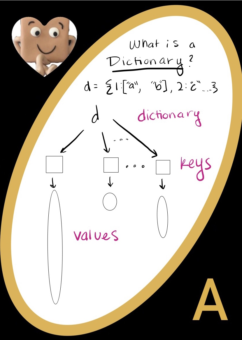
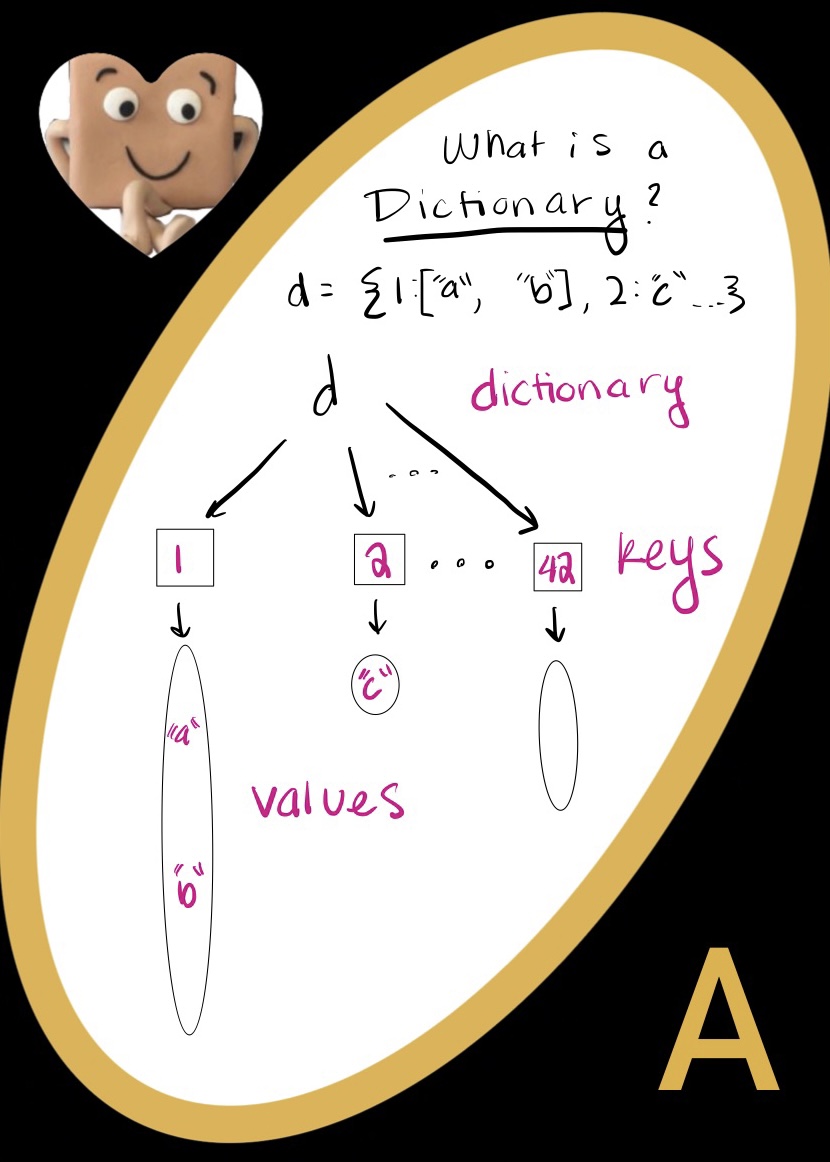
Easy to change elements in a list. For example, to make every element 42, you can simply use a L[i] = 42 statement

What is a Dictionary?

Dictionaries (also known as "objects" in some other programming languages) are a useful way to store lots of information. They are defined with curly braces. Information in a dictionary is sorted by key/value pairs. Here's an example of a dictionary:

d = {"Mudd": ["Best School", "STEM", 42], "Pomona": 47, "Pitzer": "Politics", "Scripps": "Music", "CMC": "Cash Money"}

Each entry in a dictionary follows the key: value format and are separated by a comma. Each key can only have one corresponding value in python but that value can be a list or tuple! In fact, keys and values can both have any type

vwl

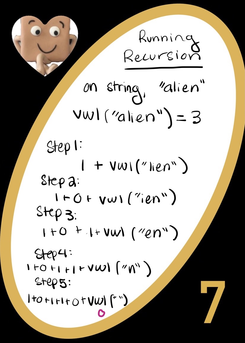
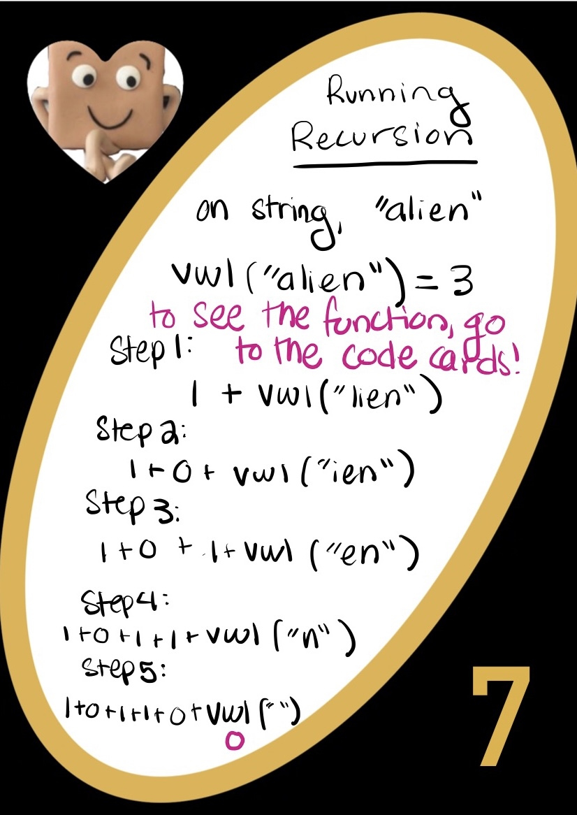
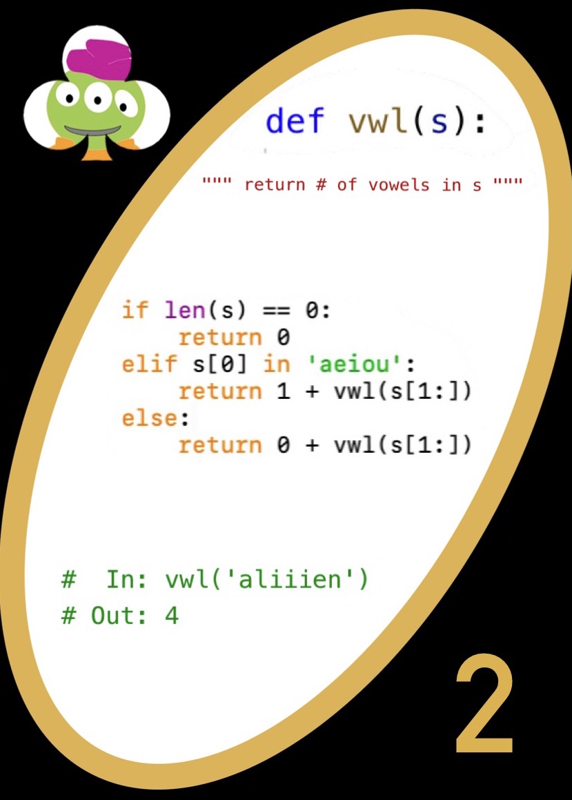
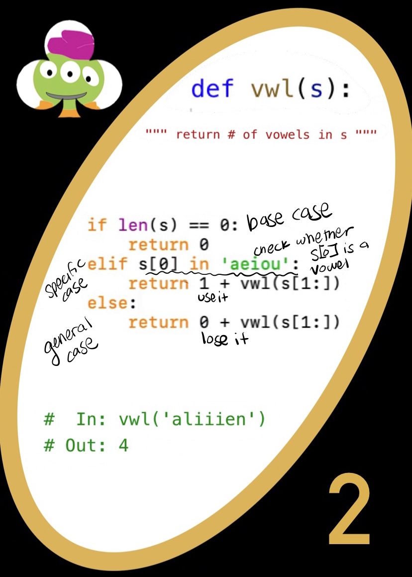
For our very first statement, we have the base case for our recursive function; if the length of the string is 0, then we return 0, which makes logical sense because how many vowels can a nonexistent word have? 0. Since there is no recursive call in this if statement, this marks the end of recursive function. The following elif statement checks if the first letter of our string is a vowel. By checking if x in “aeiou” we say the following: if the value of x can be found inside the string “aeiou”, then it is a vowel. So if x equals “e”, then the statement evaluates as true since “e” is in “aeiou”. If true, then we add one to whatever the total vowel count is for the string excluding the first letter (which we will calculate later using recursion). In other words, we know that the first letter is definitely a vowel so we know that the string has at least 1 vowel total; now we have to check the rest of the string (s[1:]) by going through the same process of

identify the first letter
check if vowel
use it by adding 1 or lose it by adding 0
recurse to check vowel count of rest of string

Finally, the last elif statement covers the case where our first letter is not a vowel; thus, we return 0 (the lose-it since we’re not returning anything substantial). Then, we continue with our day and check the rest of the string with the recursive function.

List Comprehension

The format of list comprehension goes something like this:

[ operation for element in list ]

which is a shorthand version of this:

newList = [] for element in list: newList += [ operation ] return newList

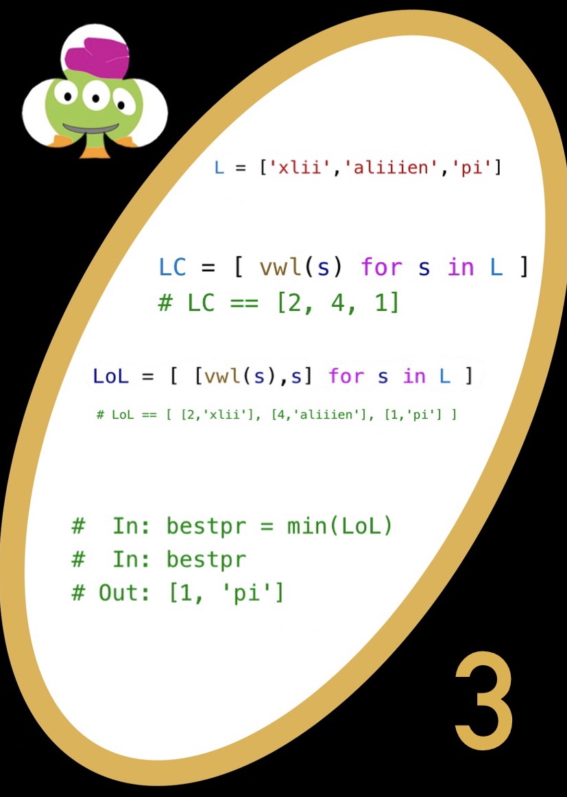
The following example

LC = [vwl(s) for s in L]

can be described as for every s (element) in L (list), we want to return the vowel count for each s (operation) which will all be stored in a new list by the end or

newList = [] for s in L: newList += [vwl(s)] return newList

Likewise, LoL can be described as for every s (element) in L (list), we want to return an array containing the vowel count in the first index and s in the second

remAll

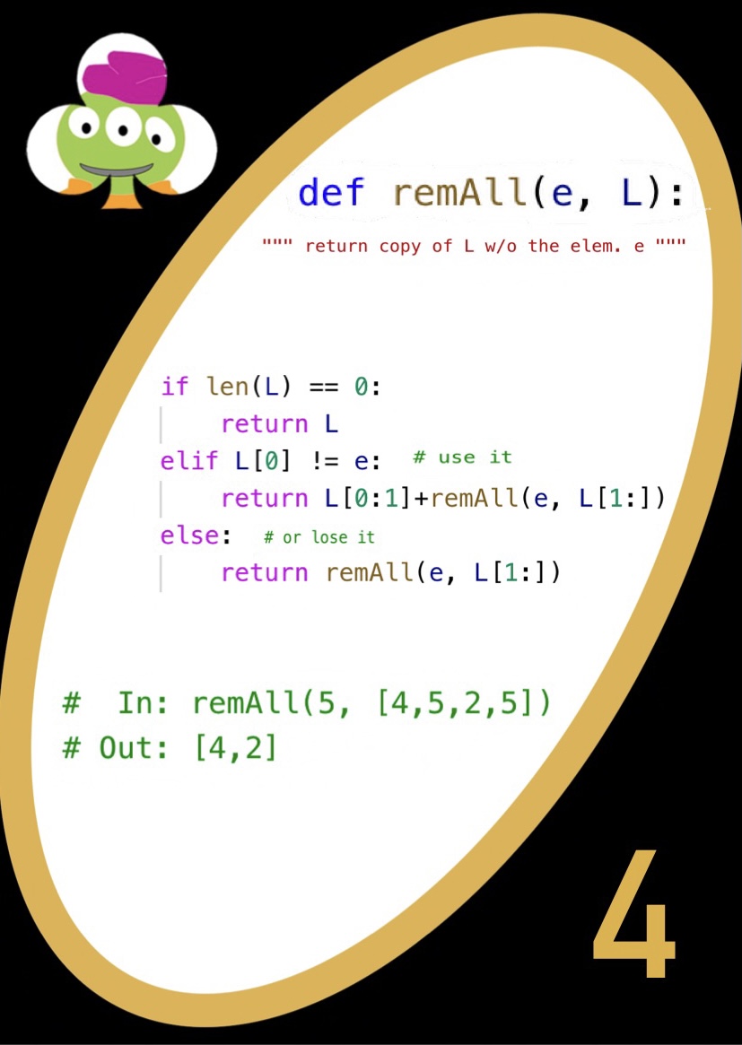
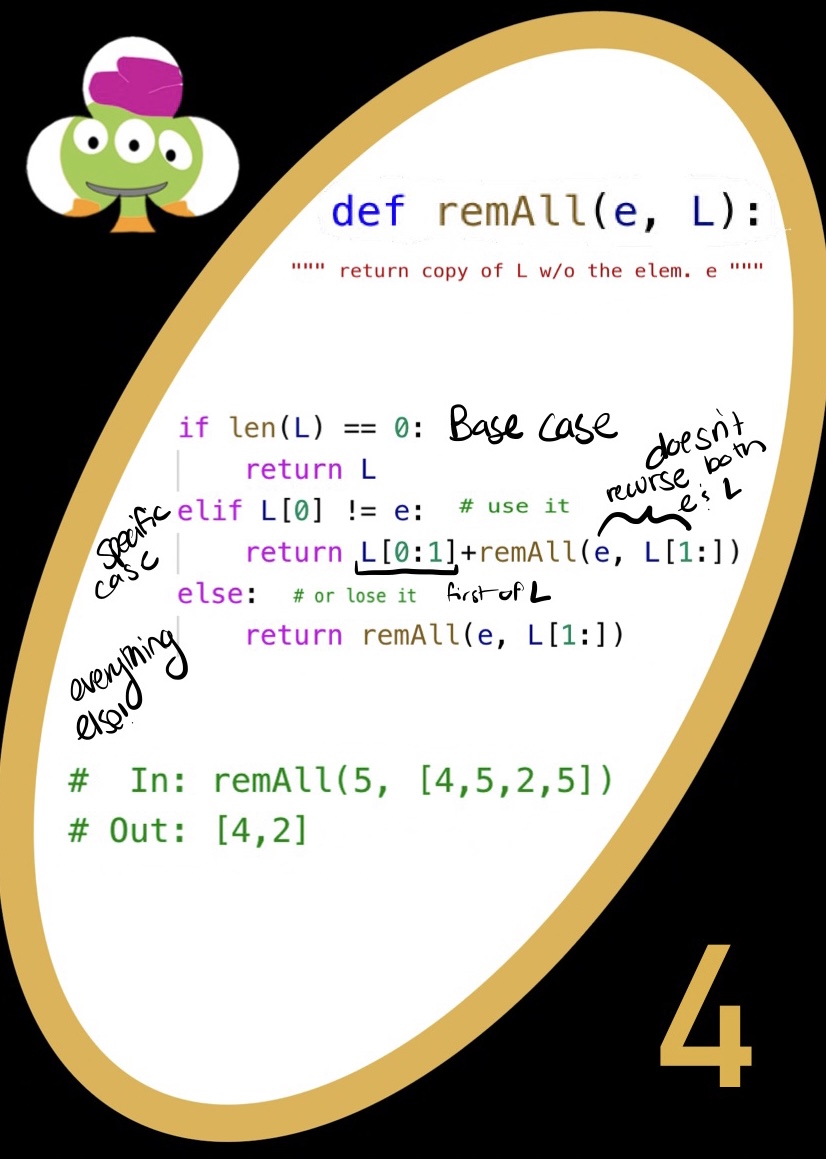
Our first if statement sets up our base case, or what will terminate our recursive function. In this case, if L is empty, then we return the empty list since an empty list does not have any elements, much less element e.

Our next statement checks that the first element of L is not equal to e, thus meaning we don’t have to remove it from the list if evaluated as true. To achieve this, we will return the first element of L which will be added to the recursive call remAll(e, L[1:]). This recursive call should return the rest of the list (not including the first element) that already has all elements e removed from it. If this is confusing, think about it like this: imagine that remAll works perfectly already. Then we know that remAll(e, L[1:]) should return a list with all e’s removed. So since we know that the rest of the list L[1:] has had all of its e’s removed, all we need to check is that first element; if it isn’t e, then we don’t have to remove it and can simply add it to the already modified list.

In the case that the first element of L is equal to e, then we simply call the recursive function without the first element. This essentially “loses” the first element of L because as you can see, we’re not returning it anywhere. We dropped the e to have our perfect e-less list.

numToBinary

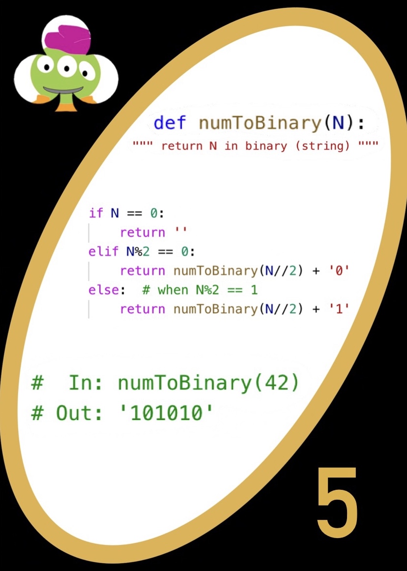
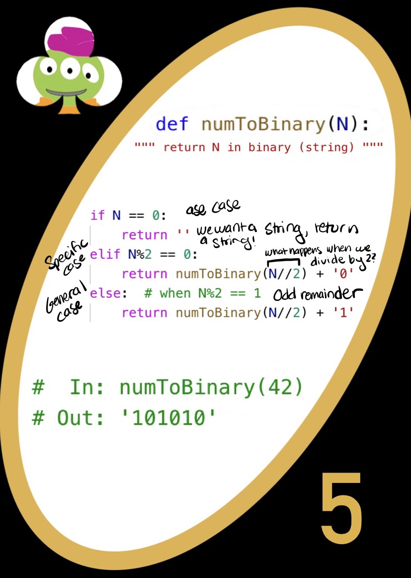
The goal of our numToBinary function is to get some integer, N, into a binary string. We can do this with recursion, even if it is a little funkier than normal recursion.

We have our main 3 elements of recursion: first, we have a base case. For the base case here, we want to check whether N is 0 (since N is an integer) and return an empty string. Why a string and not the integer 0? Well, we know that we want our function to return a string of binary digits, so any recursive shenanigans will need to be built on an object of type string, or in our case, an empty string.

Now for the second element of our recursion: our specific case. For our specific case, we are going to check whether the current number N is even. If you don’t understand why we can check N, feel free to take a look at Spam cards A,2, and 3. Well, once we are certain that our N is even (we check this by ensuring the remainder when divided by 2 is 0), we want to add a ‘0’ to our string. There are a couple of things to notice here.

We are adding the ‘0’ to the end of the recursion. We want to do this because otherwise our end result string will read backwards. This doesn’t usually matter, since we often use recursion to count things, but for this function, we want a string back.
In our recursive call of numToBinary, we are using N//2. This is different from what we normally do in recursion. Here, it is not sufficient to simply subtract 1 from N (which is normally our procedure). Instead, we want to divide by 2 so that we can get the next N, while at the same time recording the remainder. Again, spam A and spam 3 are really good resources to understand this.

Finally, we do the third element of our recursion: we consider the general case. Here, we are basically doing the same thing that we did for the specific case. The only difference is that, in binary, all things that aren’t even are odd, so any general case is just asking “is our number odd”. We then repeat the same procedure as the specific case, except now we want to add ‘1’ to our string, to signify that N has a remainder of 1 when divided by 2

evenSum

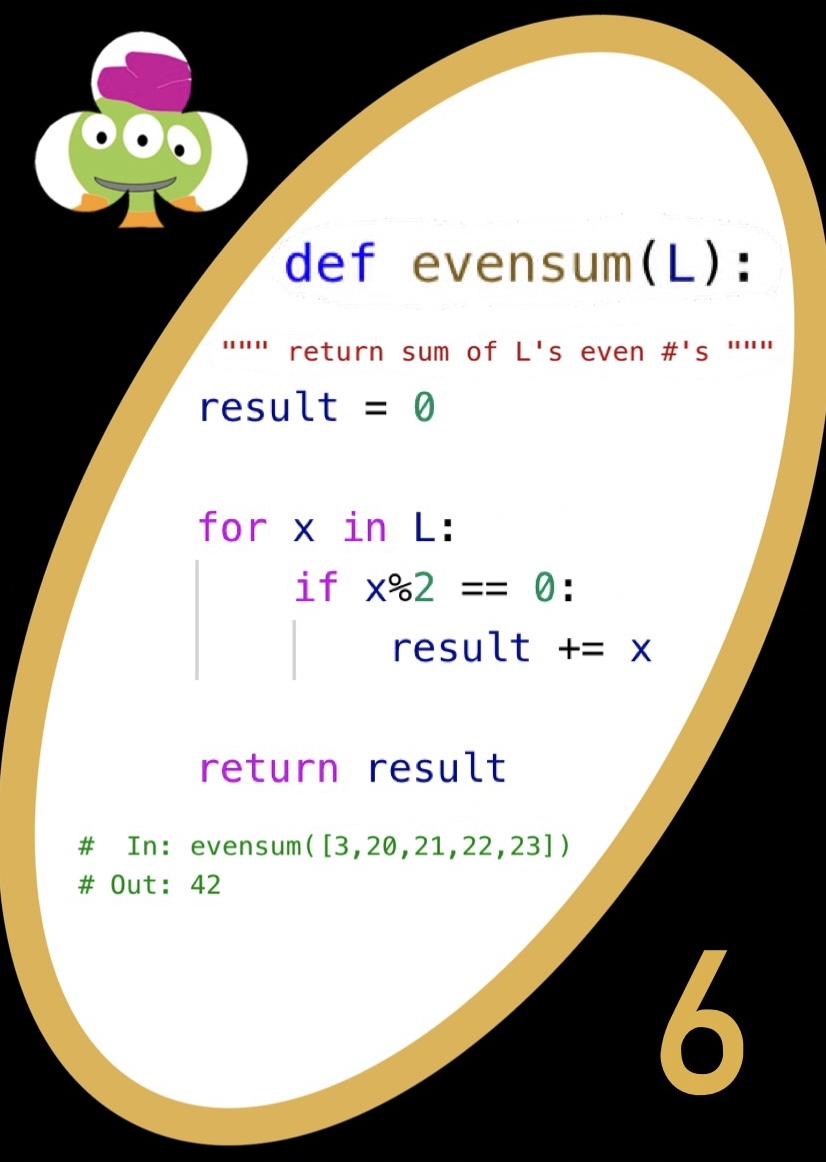
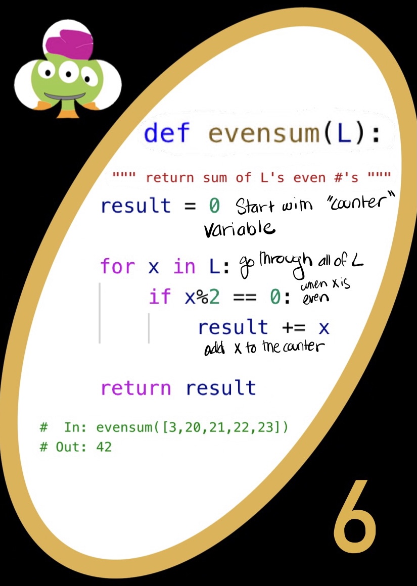
First, we want to have a counter variable which will keep track of the sum of L’s even numbers. We start at 0 because we haven’t actually added anything yet.

for x in L identifies that we’re going to be looping through the array L, where x represents each individual element of L. For example, in a list of [1, 2, 3], x will have the value of 1 in the first iteration, the value of 2 in the second, and the value of 3 in the last.

The if statement checks if x is even by asking, “If we divide this number by two, do we have a remainder?” From basic math class, we know that if it doesn’t, then it is even. If x is found to be even, then we add that number to the current value of result. The result += x is equivalent notation to result = result + x.

At the very end, we want to return result so we can see the sum of even numbers

indexofmax

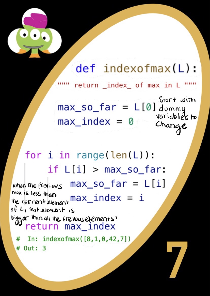
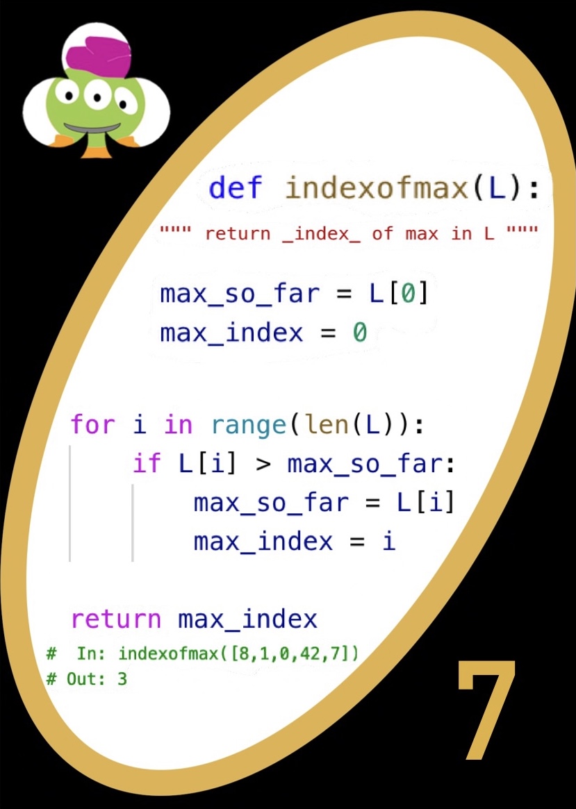
We first start by saying that the index of our max is the first element in L. We do this with our two variables max_so_far (set to L[0] to get the first element of L) and max_index (set to 0 to represent the first index). As we loop through our list, we will be updating these values.

We will be looping through the array such that i is equal to the index. This is because we set i to be the elements in the range of 0 (inclusive) to the length of L (exclusive).

Our if statement says that if the element at index i of L is greater than the max we have so far, then we must update our new max to be the current index at i. We do this by setting max_so_far to the current element with L[i], and the max_index to the current index as i. Then, we continue looping through the rest of L while repeating the “updating the max” steps. After the loop is finished, we return the index of the max element in L.

livecount

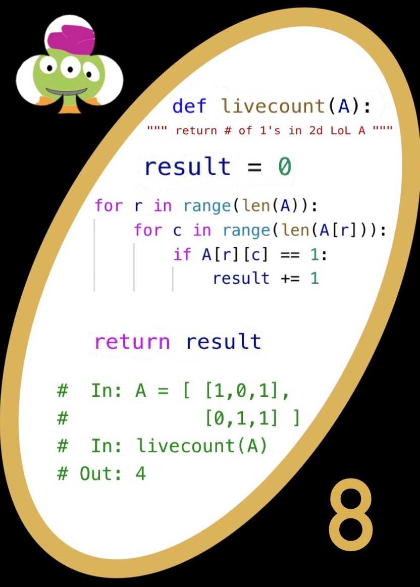
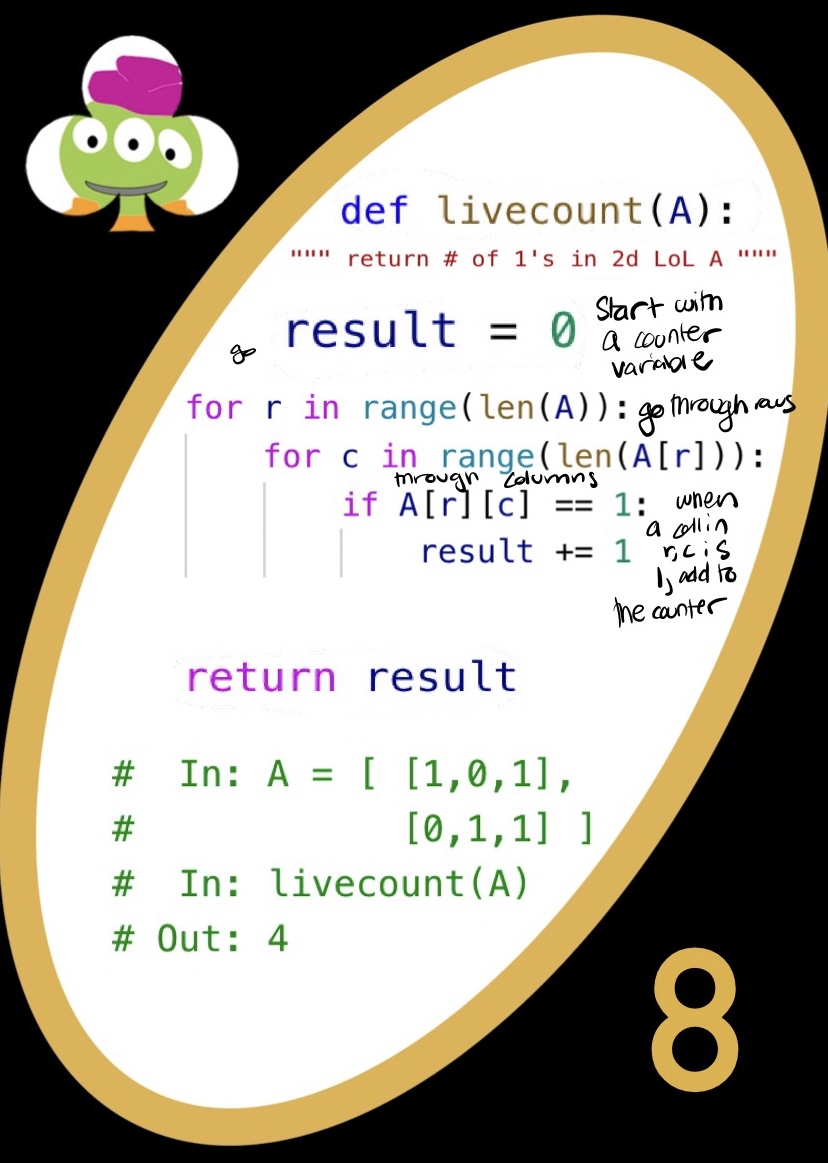
If we have a 2D LoL A, to get to any element of the LoL, we must first specify which of the inner lists we want and then which element in each of those lists we are after. This means we’re going to use two for loops: a first for loop to go through the list of lists, and a second for loop to iterate through the inner lists.

We want our code to count the number of ones in this big LoL, so we are going to start with a counter variable, “result”. This variable is going to act as storage, and every time we encounter a one in our LoL, we will add to result. This means that result is the end product we will return.

Now for the for loops. We have our two for loops: if we imagine the outer for loop iterating through all the rows and the inner for loop to be iterating through the columns, A[r][c] is just the (x,y) position of some (c,r). If this doesn’t make sense, please see Wally 9. When the LoL has a one at that (c,r) position, we add one to result. Once the for loops are done (put another way, once we have gone through the entire LoL), we return result.

allcounts

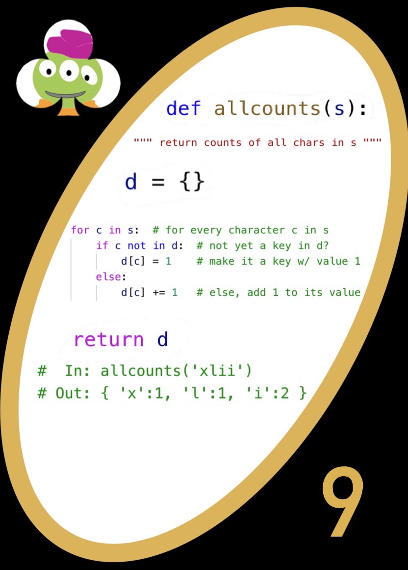
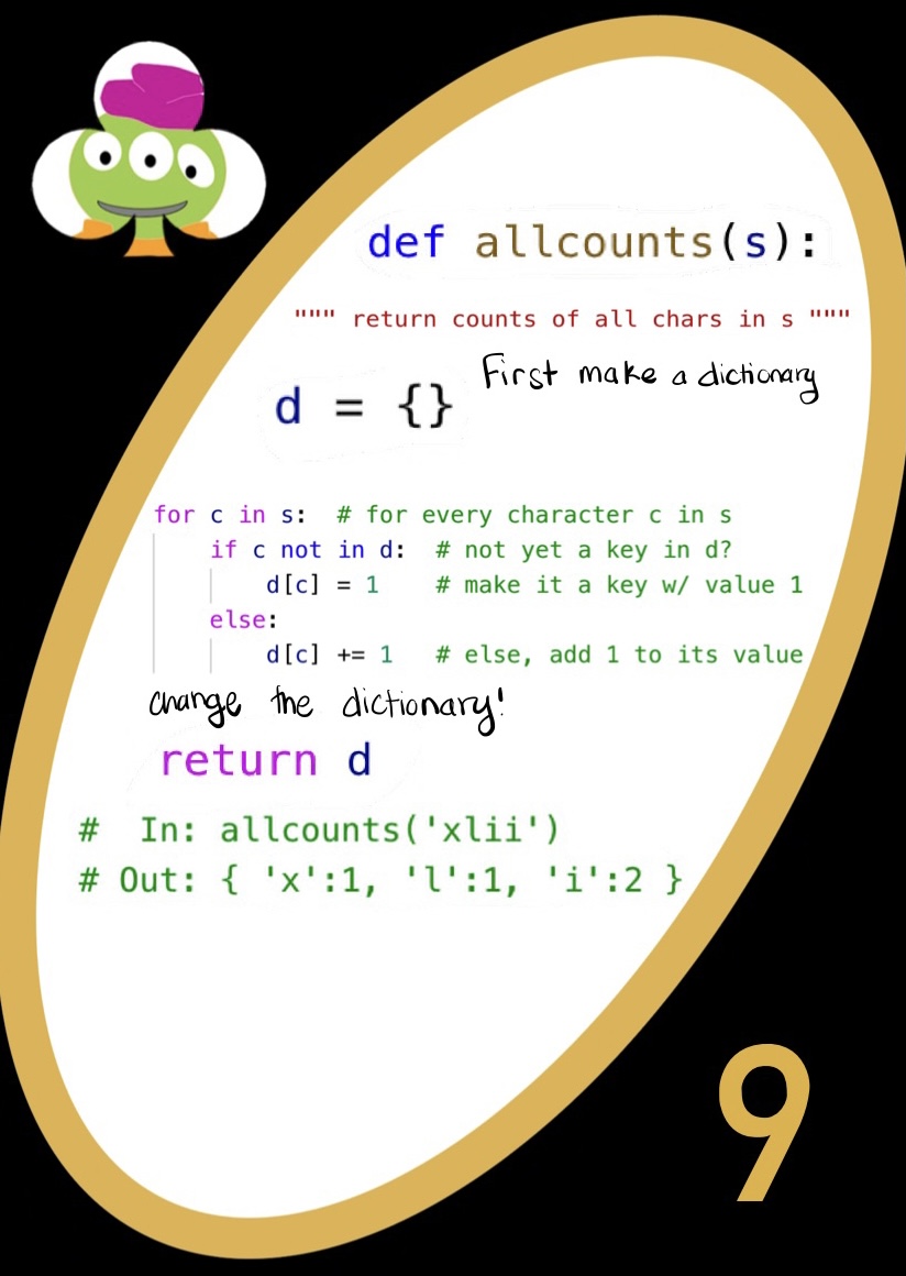
In allcounts, we want to count the characters in s. To do this, we are going to use a dictionary. To start with, we need to make an empty dictionary d. We can do this with that first line in our code.

Next, we want to go through the string s, and add new characters to the dictionary, counting old ones. We know from Wally Q and Wally A that dictionary keys can’t be repeated. Basically, we need to add ONLY new characters to the dictionary as keys. The repeated characters will already be keys, so we can just add to their values.

To do this, we can use a for loop that iterates through all the characters in our string s. Next, we need to check if the character is a key in d. We do this by asking whether the character is not in d. This may seem harder than asking “character in d”, but by checking that the character is not in d, adding characters becomes our first priority. For the flow of our code, this is better.

Once we check that a character isn’t in d, we add it by making the key correspond to the value one. This means that there is at least one character in s that we have just specified. If the character is already in d, we can just add one to the value that is already tied to the key.

In the end, we want to return d. We’re done!

Alien Class

In the alien class, we can see the three main parts that we talk about in our Spam J: What’s in a Class?!. First, we have the constructor. Then, there’s the repr function. Finally, we have a method called addEyes. To make the aliens tea, fea, and ftea, we get to call the Alien class. Let’s break down what each block of code does:

The constructor

Takes in “self”, or the specific object that we have yet to make, and ne, which gets assigned to the number of eyes that the alien has.
Makes the Alien object that has the numeyes attribute

The repr

Also takes in “self”
Returns the string representation of the Alien object, which is specified by how many i’s there are in alien.

The method, addEyes

Takes in “self” and the ni to add
addEyes changes the attribute

Undebuggable Functions

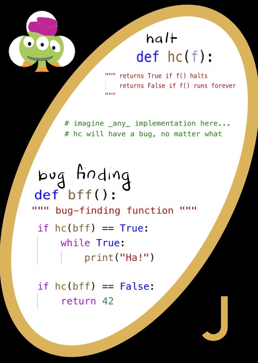
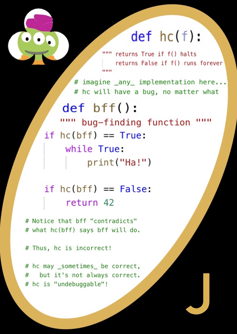
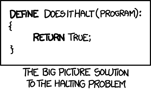
The easiest way to think about this dilemma is to use an example function. Suppose bff halts. Then hc(bff) will return True. However, when we run bff, we see that if hc(bff) is True, we run a while loop that runs forever! Therefore, bff will run forever. This directly contradicts what we said earlier.

Let’s do one more example run. Suppose bff runs forever. Then hc(bff) should return False. However, in bff, if hc(bff) is False, bff halts! This contradicts our assumption that bff runs forever.

Get the picture? Whatever we decide bff should do (halt/run forever), we end up getting the opposite when we actually consider the bff and hc functions together. In essence, we have created an impossible situation for ourselves: hc is undebuggable.

Minterm Circuit

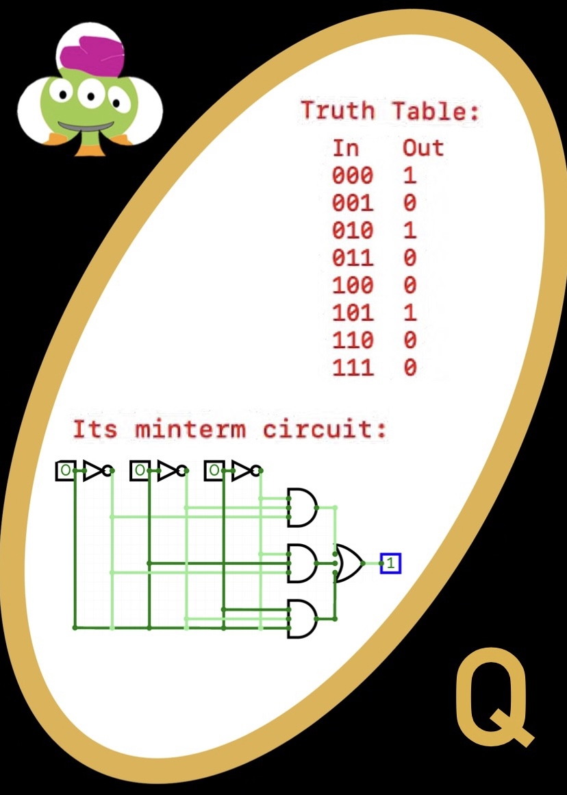
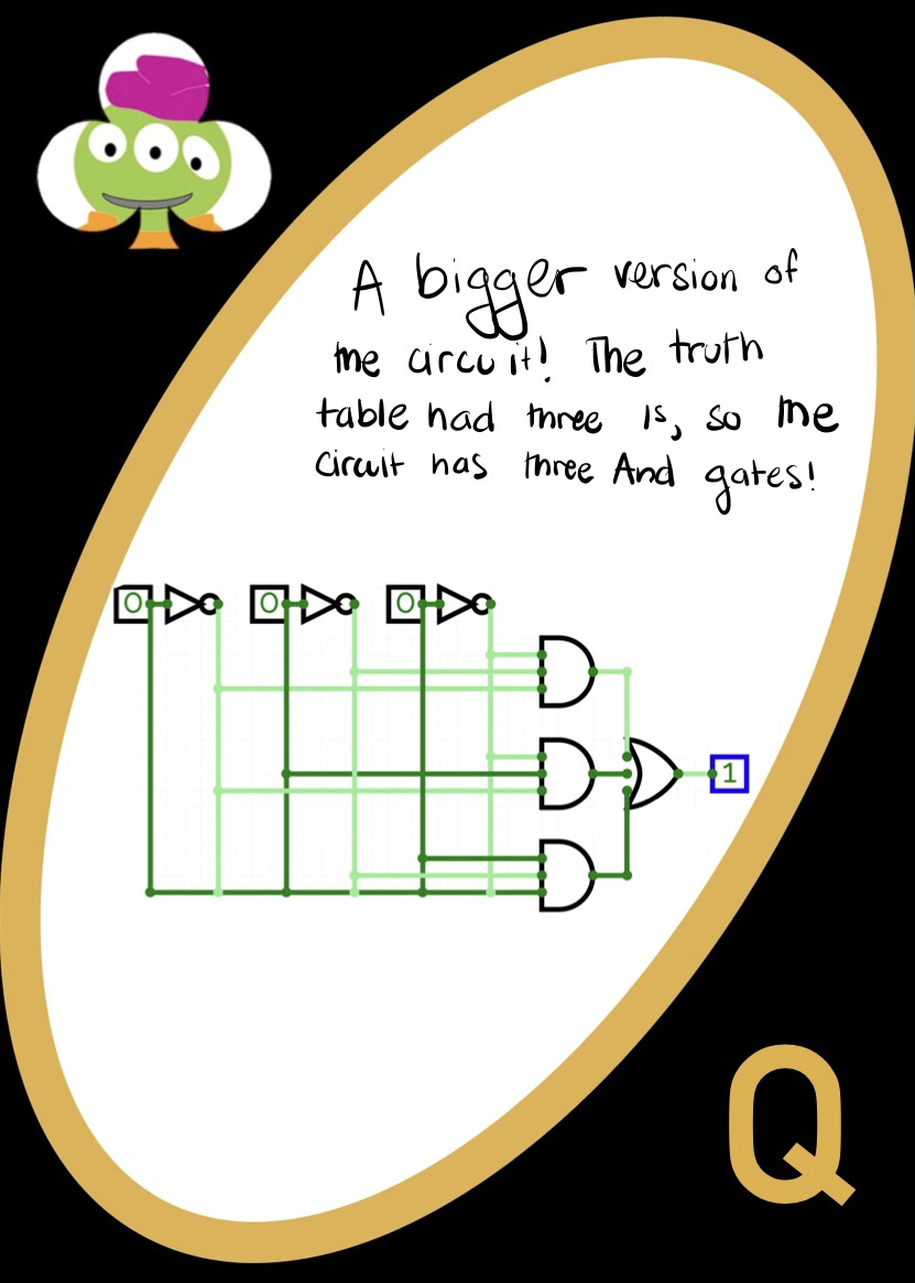
Whenever we have a complete truth table, from Spam 5, we know that there will be at most as many And gates in the circuit as there are ones in the output column. In our card example, we have no idea what the big picture concept for this circuit is, so we are going to have to make our circuit “blindly” from the truth table.

To start, we know that there will only ever be three inputs. We can add these to our circuit, with Not gates. We also know that there will be three And gates, each taking in three inputs, and putting out one output. We know this because each And gate will need to consider all the inputs in each case. These And gates will be connected by an Or gate, and then to the output.

From there, we can simply connect the And gate inputs to the corresponding input digits. When any of our three And gates gets an input that returns true, we will get a one for an output.

Finite State Machines

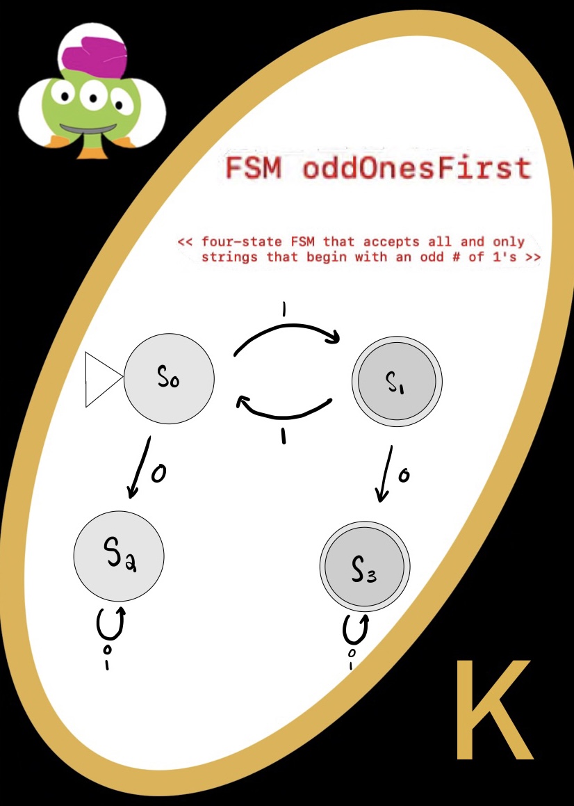
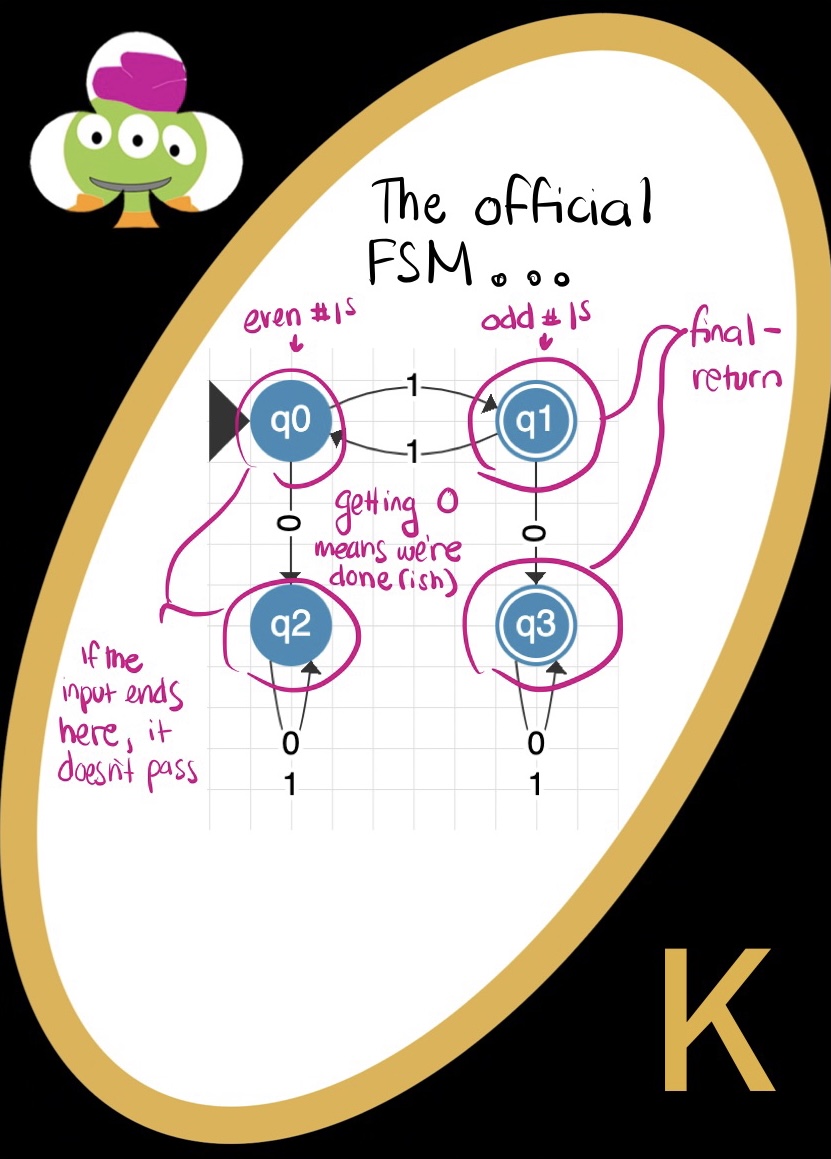
oddOnesFirst asks us to to design a FSM that accepts strings with an odd number of ones first. Since we are counting ones/zeros, we can make an imaginary grid: moving along states to the right means we are adding ones to our string, and moving down means we are adding zeros.We’re confined to only 4 states: so we can break our FSM down to it’s main parts. First, we need a start state. We can imagine that this state is when we have zero ones and zero zeros. Since zero is even, we want strings that end here to be rejected.

The next state we may want is our state to count ones. On a basic level, if we count one one, without any beginning zeros, we want strings to be accepted. Then, we know that our first state (q0) will send to q1 if our string starts as a one. If q1 gets a one, though, we know that we will have counted two beginning ones. That means we should send our string back to the “zero ones” or q0 case. Wow! We’ve done the hardest part, handling even and oddness!

The next consideration for us is one that we have so far ignored: what do we do with zeros? Well, we know two main things: first, if our string starts with a zero, we want to reject it. Second, if our string goes to a zero after a certain number of ones, we want it to stay in whatever state it was in when we counted the ones (ie, if we get 1001 it should accept, and if we get 11001 it should reject). We will need two states for this. The first, q2, should reject when we get a zero after an even number of ones. This means that if we get a zero from q0, we should move to q2, and stay there. On the other hand, q3 should accept if we’ve had an odd number of ones so far. So, if we get a zero from q1, we want to go to q3 and stay there, no matter what.

Now that we’ve made four states, we’re done! If you’re still confused, have no fear - visit Spam 7

if/elif/else

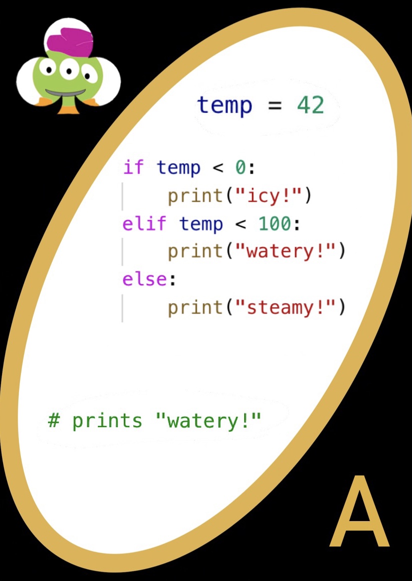
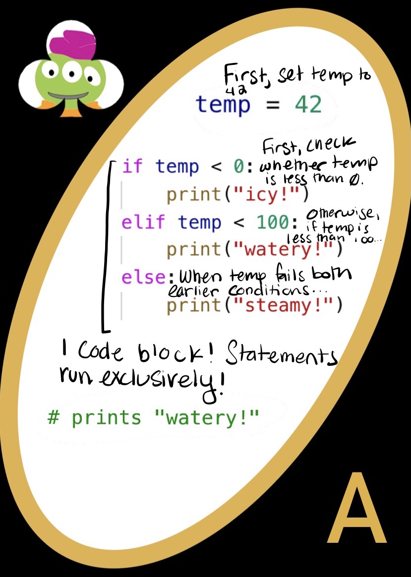
Walking through this code, we can see a couple major takeaways.

First, the thing we are checking in each of our if/elif/else statements is the “temp” variable. By saying temp = 42 at the beginning of our code, we are telling our python to store the integer 42 in the variable temp. Every time we print temp> or compare temp> to something else, we are really comparing it’s value, 42
The second big takeaway is in the if/elif/else statements. We first have an if statement: this if statement is checked first. The elif statement is paired with the if statement, so the elif is checked only when the if statement does not return True. The same is true for the else statement, except that it is after the elif statement(s)

In our code, temp> (or 42) is not less than 0. We then move on to the elif statement. Since 42 is less than 100, we print “watery!”. We ran one of the linked statements, so the code doesn’t consider the else case. If we instead had two if statements, an elif, and an else, the two if statements would both be checked. That is, an if/elif/else block is exclusive